Week 1- Mixing Tee
SIMULATION OF MIXING TEE USING ANSYS FLUENT
Aim:-
To set up steady-state simulations to compare the mixing the effectiveness when the hot inlet temperature is 36°C and cold inlet at 19°C.
Introduction:-
The mixing tee simulation is used in the air conditioning system to get the desired output temperature. The mixing characterizes the phenomenon where hot and cold flow streams join, mix and result in temperature fluctuations.
Theory:-
- In this challenge, to simulate the mixing tee of two different lengths.
- The Hot inlet temperature is 36°C and the Cold inlet is at 19°C.
- Use K - Epsilon and K- Omega SST model for the first case and select a more suitable model for further cases.
Case 1:
- Short mixing tee with a hot inlet velocity of 3 `m//s`
- Momentum ratio of 2,4.
Case 1:
- Long mixing tee with a hot inlet velocity of 3 `m//s`
- Momentum ratio of 2,4.
Momentum ratio = Velocity at cold inlet/ Velocity at the hot inlet
In the table, comparing the following values for both cases.
- Cell Count
- Average Outlet Temperature
- Number of Iteration for convergence
Expected Result:
- Velocity and Temperature Contour plot on the cut planes along and across the pipe.
- Velocity and Temperature line plot along and across the length of the pipe.
- Perform Mesh Independence study for case 1.
- Discuss the effect of length and momentum ratio on results.
Steady State:-
Steady-state simulation computes the fully developed solution that does not change in time. When steady-steady used the mean values are computed. The steady-state simulation is way faster than transient.
To find the cold inlet velocity:-
Velocity at cold inlet = Momentum Ratio `xx` Velocity at hot Inlet
If Momentum ratio is = 2,
Velocity at cold inlet = 2 x 3 `rArr` 6 `m//s`
Velocity at cold inlet = 6 `m//s`
If Momentum ratio is = 4,
Velocity at cold inlet = 4 x 3 `rArr` 12 `m//s`
Velocity at cold inlet = 12 `m//s`
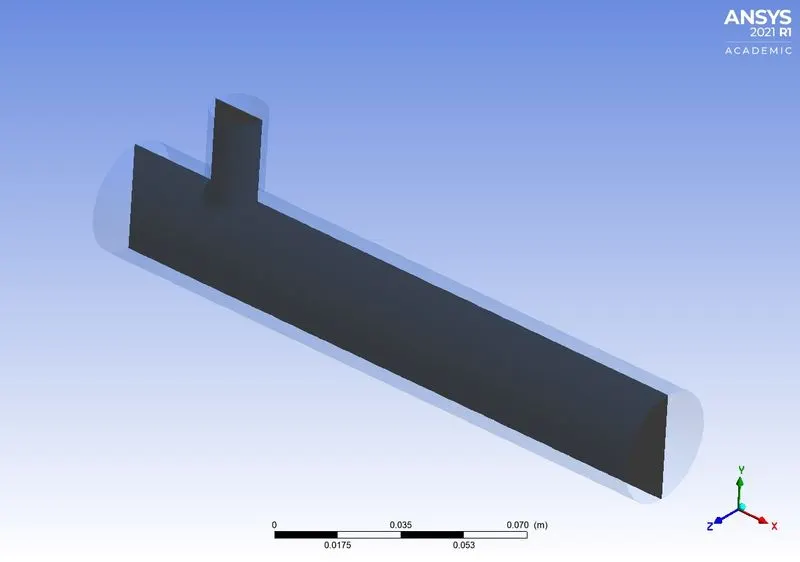
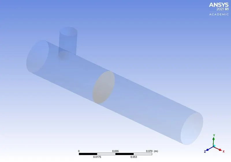
Creating cut plane along and across the pipe:-
The plane is used as a location to create a contour plot.
1. Short Mixing Tee
2. Long Mixing Tee
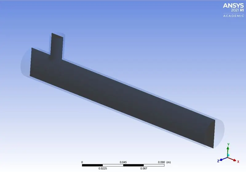
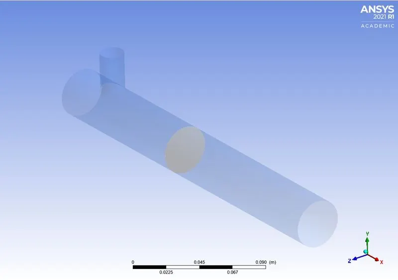
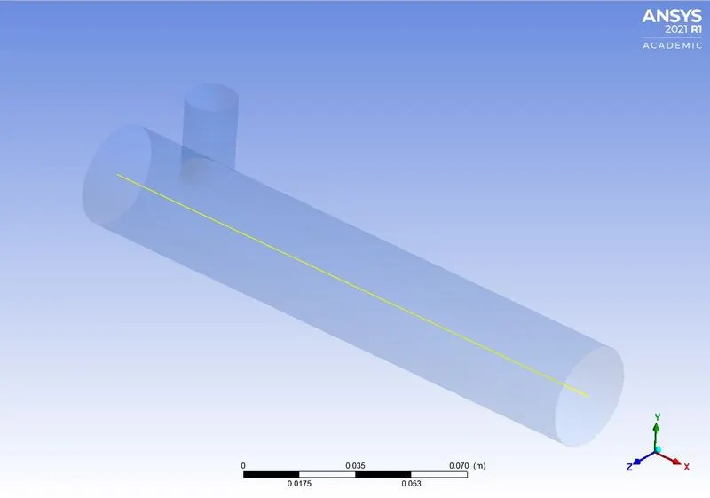
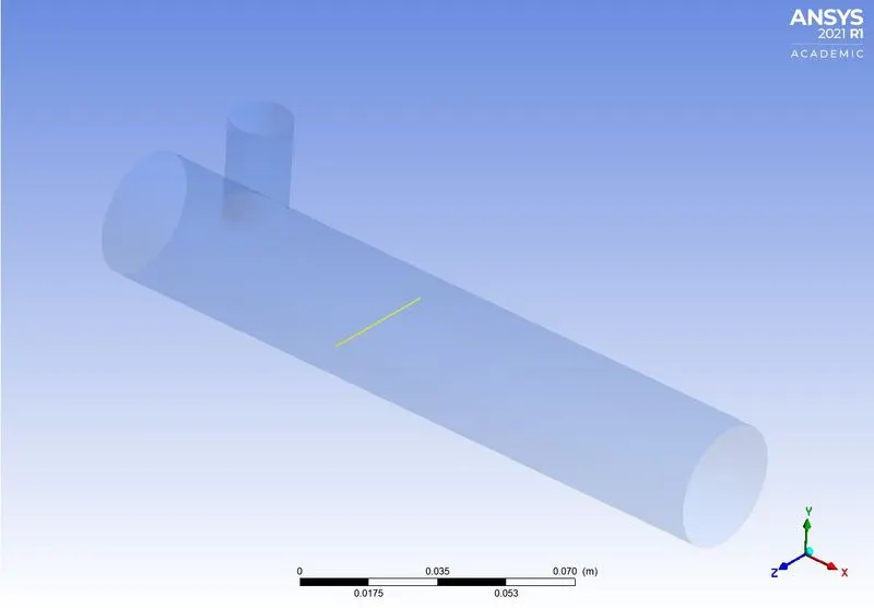
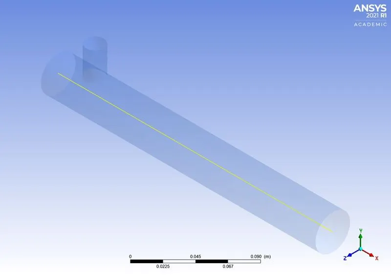
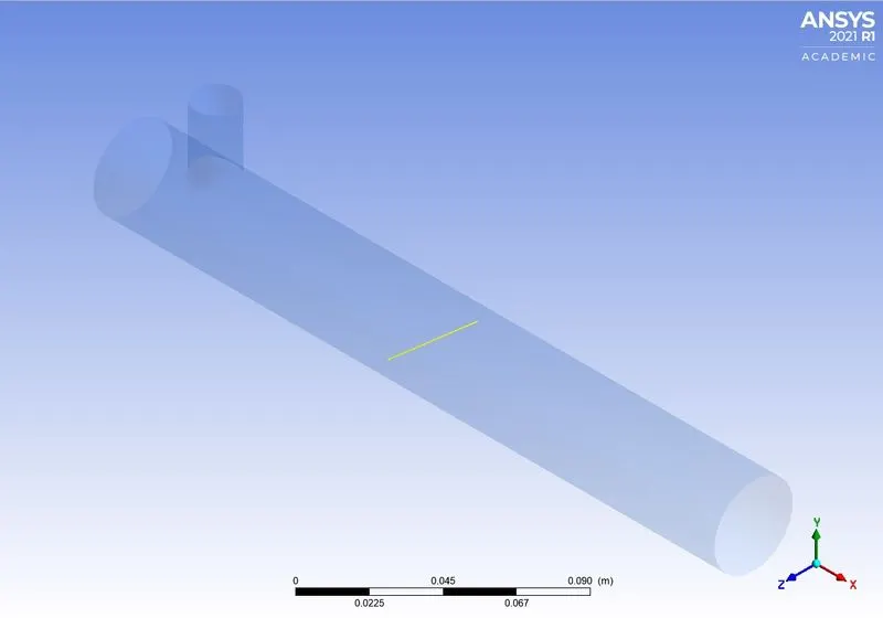
Creating line along and across the pipe for line plot:-
The line is used as a data series for creating a line plot.
1. Short Mixing Tee
2. Long Mixing Tee
Named Selection for the geometry using Face selection:-
The Named selection of Inlet x, Inlet y, outlet, and Walls are created in the meshing for boundary conditions.
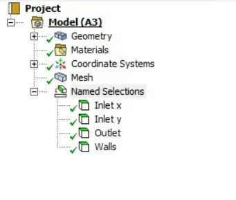
MODELLING APPROACH, PRE-PROCESSING, & SOLVER SETTING:-
CASE- 1 (SHORT MIXING TEE):-
In this case, simulating the mixing tee of short length with the momentum ratio of 2 and 4. And the K - Epsilon and K - Omega SST Turbulence model is used to find the differences.
- K-Epsilon model of Momentum ratio - 2
- K-Epsilon model of Momentum ratio - 4
- K-Omega model of Momentum ratio - 2
- K-Omega model of Momentum ratio - 4
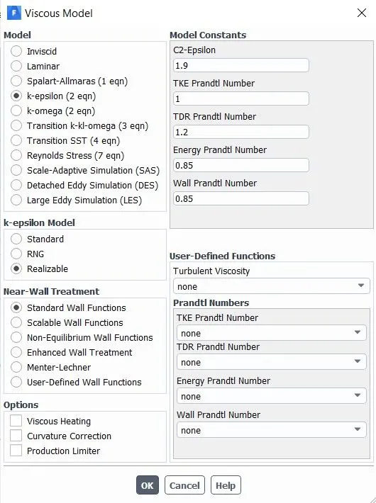
Turbulence Model:-
1. K - Epsilon
K - epsilon turbulence model is the most common model used in Computational Fluid Dynamics to simulate mean flow characteristics for turbulence flow conditions. It is a two equation model that gives a general description of turbulence by means of two transport equations (PDEs). The original impetus for the K-epsilon model was to improve the mixing-length model, as well as to find an alternative to algebraically prescribing turbulent length scales in moderate to high complexity flows.
2. K - Omega
The K - omega turbulence model is a common two equation turbulence model, that is used as an approximation for the Reynolds-averaged Navier-Strokes equations(RANS equations). The model attempts to predict turbulence by two partial differential equation for two variables, k, and ω, with the first variable being the turbulence kinetic energy (k) while the second (ω) is the specific rate of dissipation(of the turbulence kinetic energy k into internal thermal energy).
GEOMETRY MODEL:-
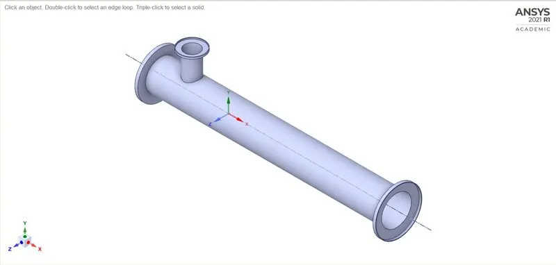
Fig 1: The geometry of a short mixing tee.
Volume Extract using SpaceClaim:
The flow volume is extracted from the geometry by SpaceClaim in ANSYS Fluent to measure the pipe's mixing effectiveness.
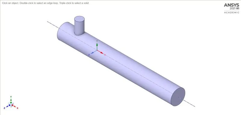
Fig 2: The volume extracted geometry.
1. K-Epsilon model of Momentum ratio-2.
MESHING:-
For getting the finer solution the mesh independence study has been getting placed. so the element size should be varied in the meshing to select the suitable one.
- Element Size = 5mm
- Element Size = 4mm
- Element Size = 2mm
Mesh Metric:
The model is meshed using ANSYS Mesher with the above element size. And give the named selection for inlet, outlet, and Walls.
1. Element size is 5mm.
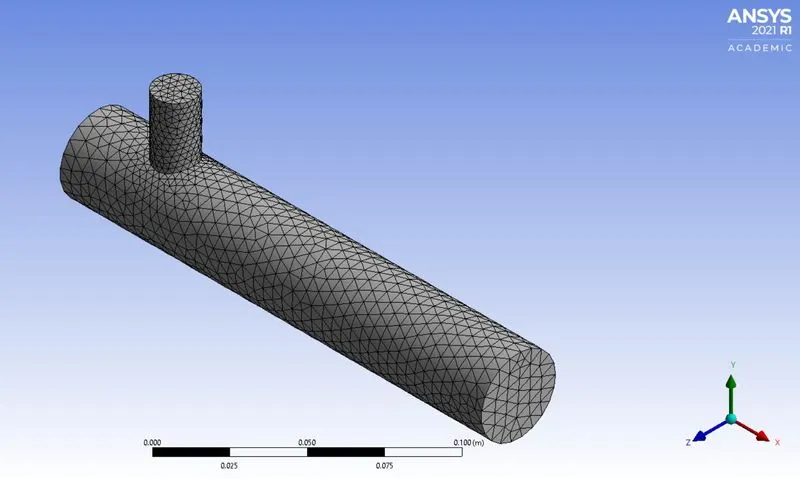
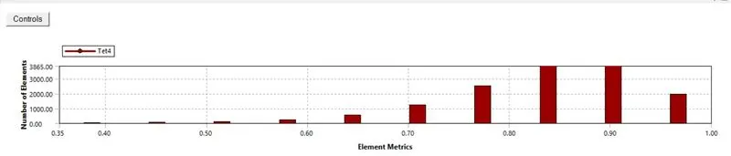
Element Quality:
- Minimum = 0.35401
- Maximum = 0.99998
- Average = 0.83697
- Std.Deviation = 9.49e-2
2. Element Size is 4mm.
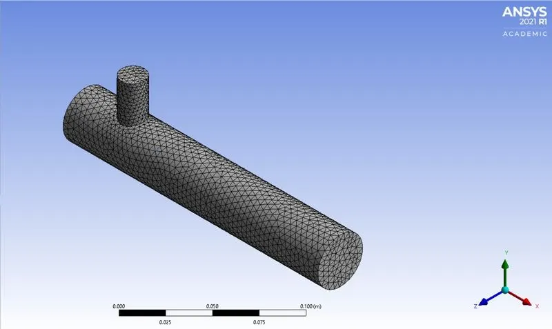
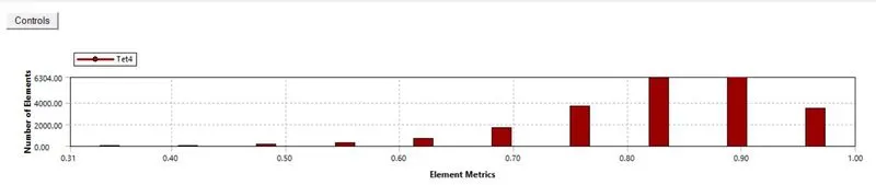
Element Quality:
- Minimum = 0.31045
- Maximum = 0.99998
- Average = 0.8351
- Std.Deviation = 9.53e-2
3. Element Size is 2mm.
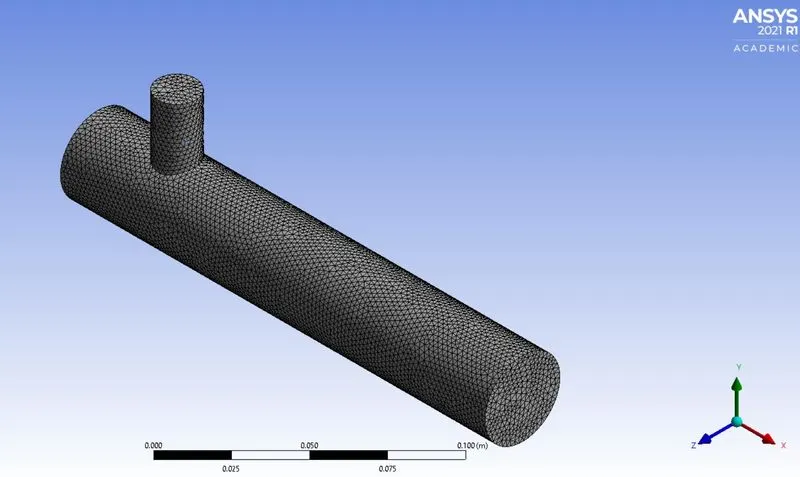
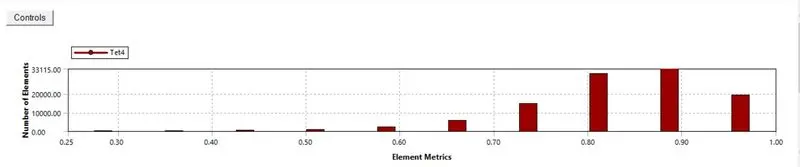
Element Quality:
- Minimum = 0.24659
- Maximum = 1
- Average = 0.83688
- Std.Deviation = 9.4e-2
Temperature Contour:-
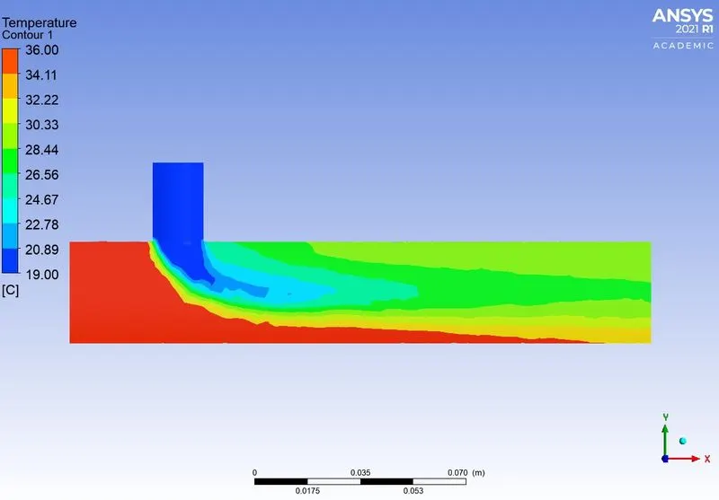
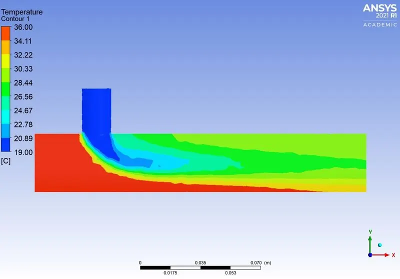
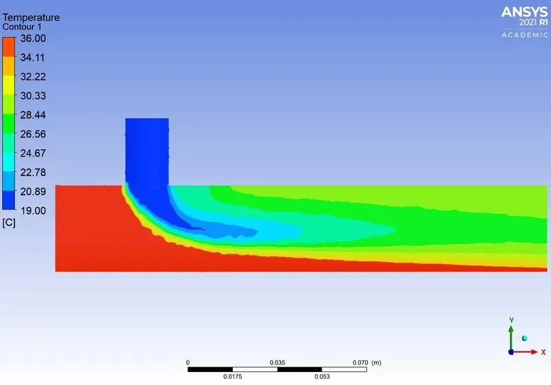
Fig(a): Element size = 5 mm Fig(b): Element size = 4 mm Fig(c): Element size = 2 mm
Velocity Contour:-
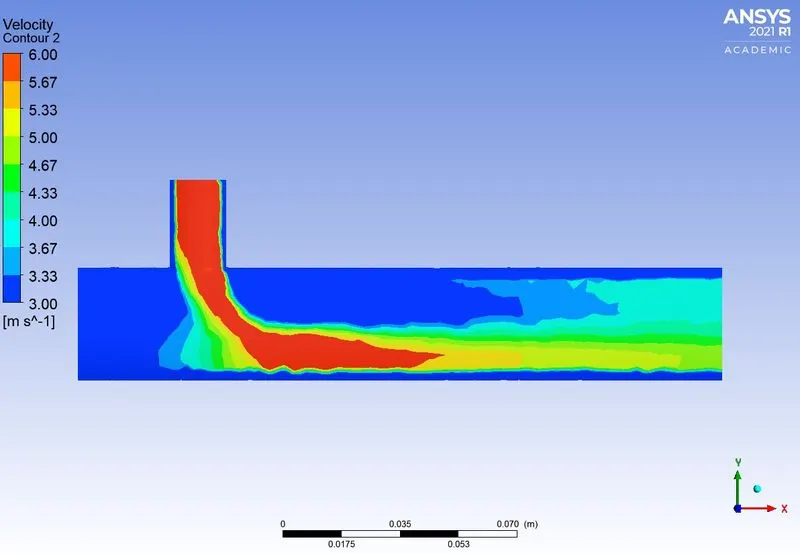
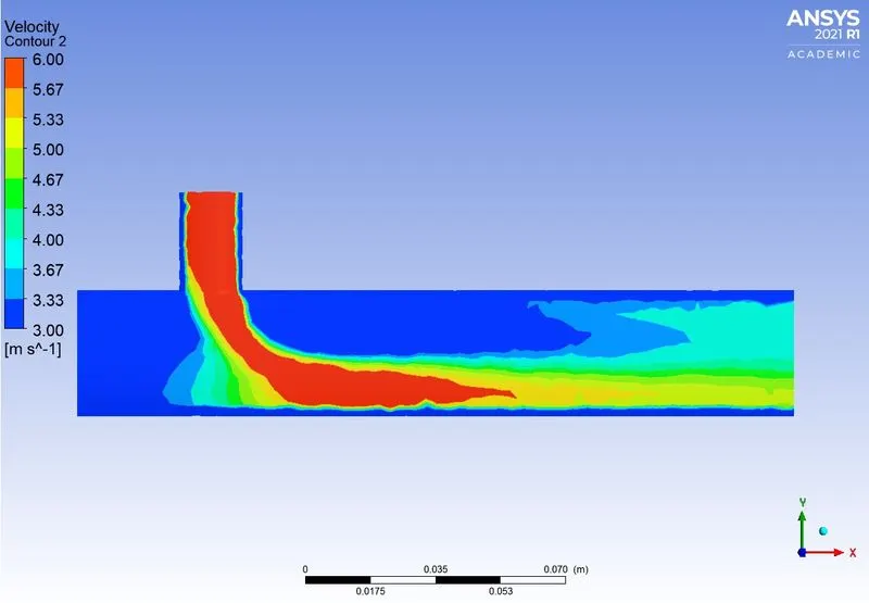
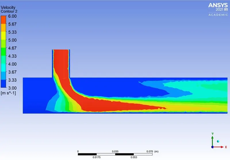
Fig(a): Element size = 5 mm Fig(b): Element size = 4 mm Fig(c): Element size = 2 mm
From the above temperature and velocity contour plot,
The element size of 2 mm gives the better quality of the mesh. So for further simulation, the element size of 2 mm is used.
SETUP FLUENT:-
From the setup to set the solver, turbulence model, and other physics.
Solver:
Type = Pressure based
Time = Steady
Velocity Formulation = Absolute
Viscous Model:
Boundaries:
1. Inlet x (Hot inlet)
Velocity Magnitude = 3m/s.
Temperature = 36°C
2. Inlet y (cold inlet)
Velocity Magnitude = 6m/s.
Temperature = 19°C
Report Definitions :
- Area-Weighted average of temperature
- Standard Deviation of temperature
Run the Calculation:
No. of Iteration = 400
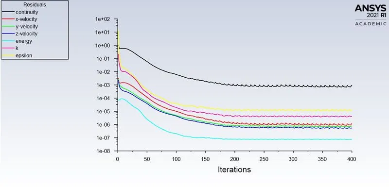
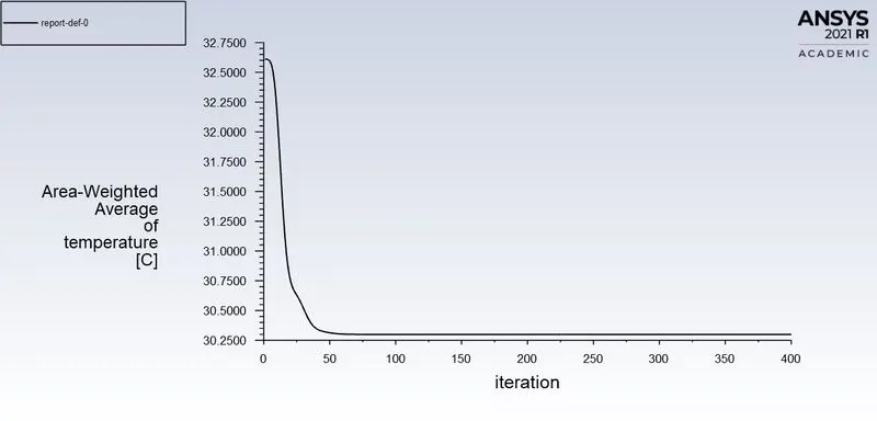
Fig(1): Residuals Plot Fig(2): Area-Weighted Average plot
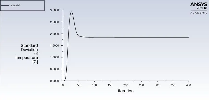
Fig(3): Standard Deviation plot
From the graph,
- The flow is converged after the 120 iterations.
- The Average Outlet temperature is 30.299281°C
- The Simulation time is 343.456 sec
POST-PROCESSING RESULT:-
1. Temperature Contour plot on the cut planes along and across the pipe.
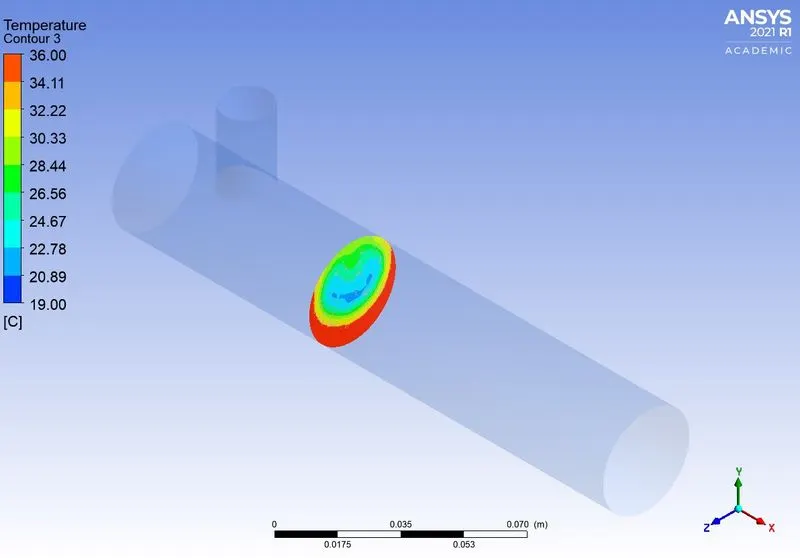
Fig(a): Temperature Contour Along the XY plane. Fig(b): Temperature Contour Across the YZ plane.
2. Velocity Contour plot on the cut planes along and across the pipe.
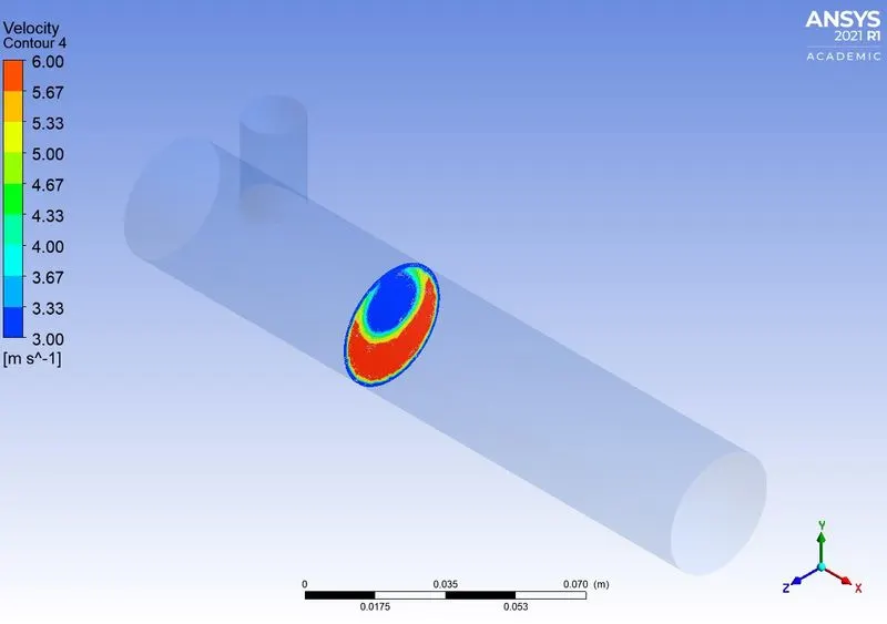
Fig(c): Velocity Contour along the XY plane. Fig(d): Velocity Contour Across the YZ plane.
3. Temperature line plot along and across the length of the pipe.
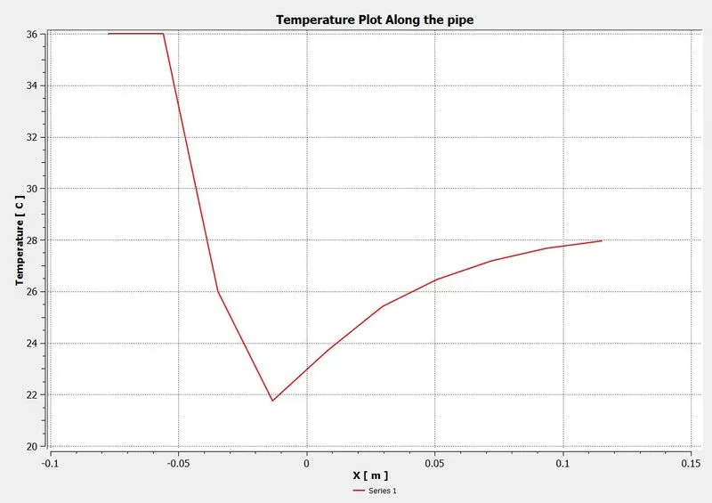
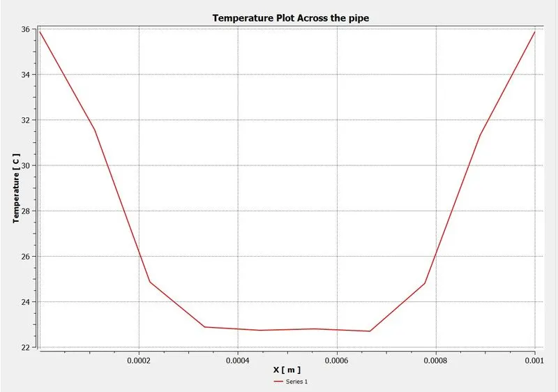
Fig(e): Temperature Plot Along the pipe. Fig(f): Temperature Plot Across the pipe.
4. Velocity line plot along and across the length of the pipe.
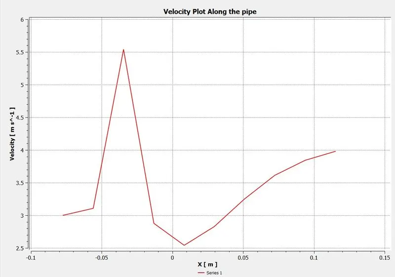
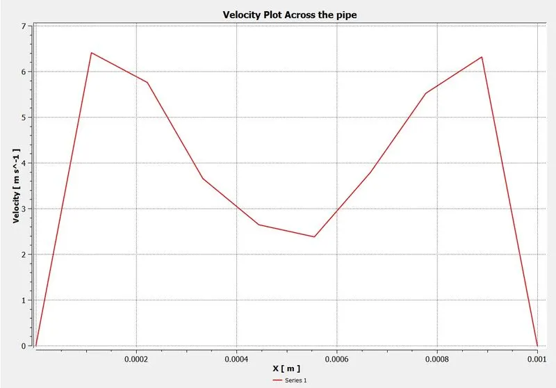
Fig(g): Velocity Plot Along the pipe. Fig(h): Velocity Plot Across the pipe.
//*****************************************************************************************************************************************************\\
2. K-Epsilon model of Momentum ratio - 4.
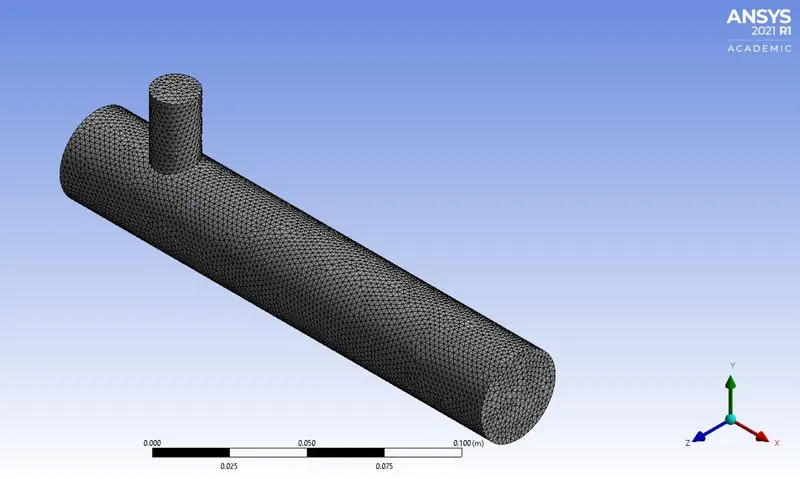
MESHING:-
The model is meshed using ANSYS Mesher with the above element size. And give the named selection for inlet, outlet, and Walls.
Element size = 2 mm
Mesh Metric:
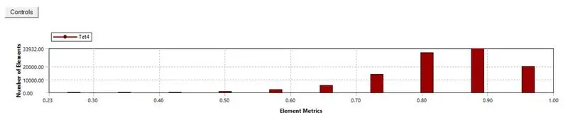
Element Quality:
- Minimum = 0.23159
- Maximum = 1
- Average = 0.83717
- Std.Deviation = 9.4e-2
SETUP FLUENT:-
From the setup to set the solver, turbulence model, and other physics.
Solver:
Type = Pressure based
Time = Steady
Velocity Formulation = Absolute
Viscous Model:
Boundaries:
1. Inlet x (Hot inlet)
Velocity Magnitude = 3 m/s.
Temperature = 36°C
2. Inlet y (cold inlet)
Velocity Magnitude = 12 m/s.
Temperature = 19°C
Report Definitions :
- Area-Weighted average of temperature
- Standard Deviation of temperature
Run the Calculation:
No. of Iteration = 400
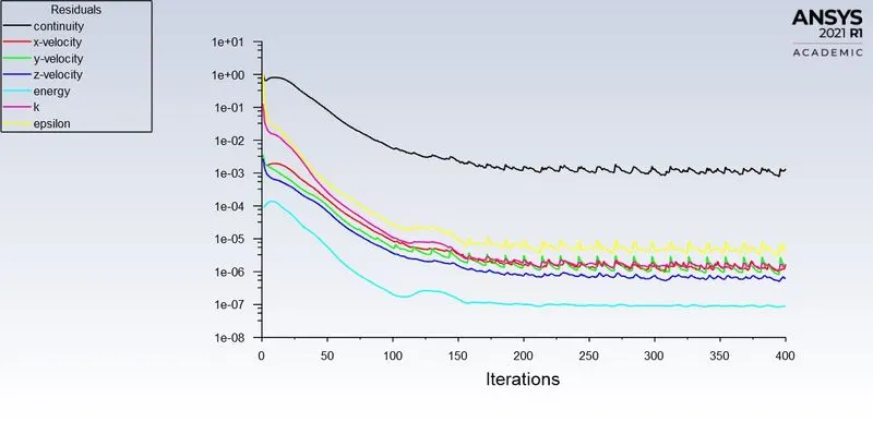
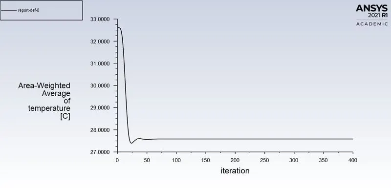
Fig(1): Residuals Plot Fig(2): Area-Weighted Average plot
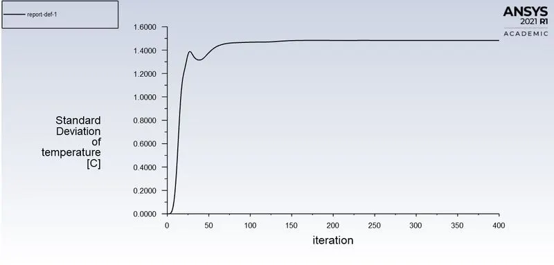
Fig(3): Standard Deviation Plot
From the graph,
- The flow is converged after the 155 iterations.
- The Average Outlet temperature is 27.586247°C
- The Simulation time is 353.377 sec.
POST-PROCESSING RESULT:-
1. Temperature Contour plot on the cut planes along and across the pipe.
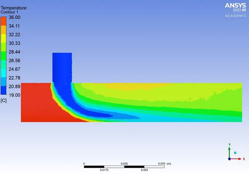
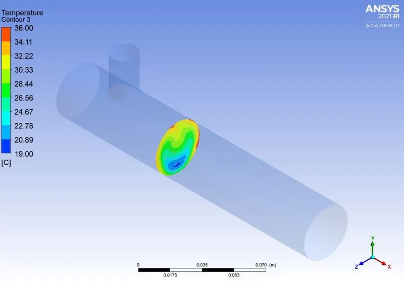
Fig(a): Temperature Contour Along the XY plane. Fig(b): Temperature Contour Across the YZ plane.
2. Velocity Contour plot on the cut planes along and across the pipe.
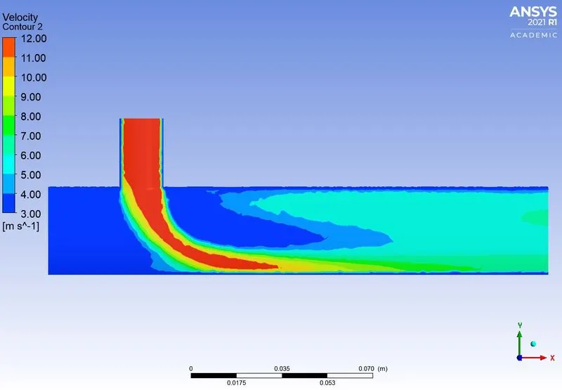
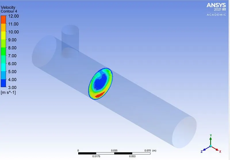
Fig(c): Velocity Contour along the XY plane. Fig(d): Velocity Contour Across the YZ plane.
3. Temperature line plot along and across the length of the pipe.
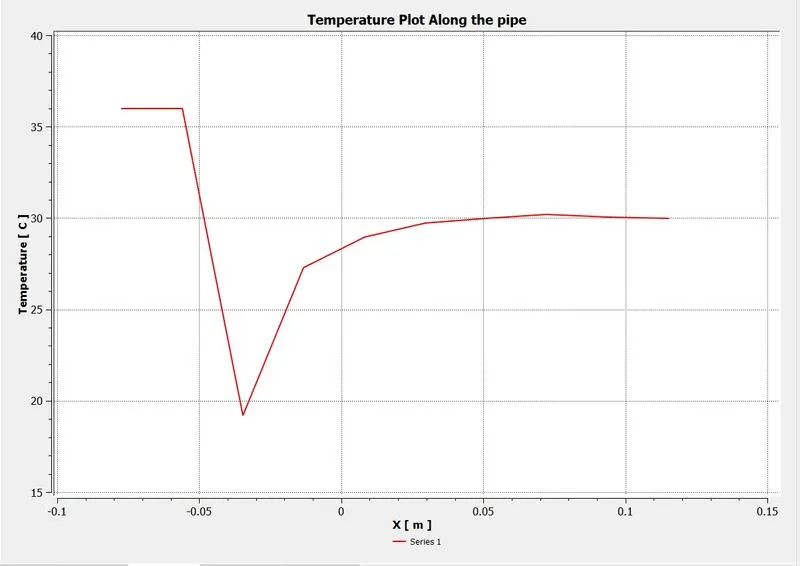
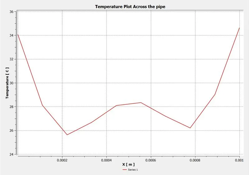
Fig(e): Temperature Plot Along the pipe. Fig(f): Temperature Plot Across the pipe.
4. Velocity line plot along and across the length of the pipe.
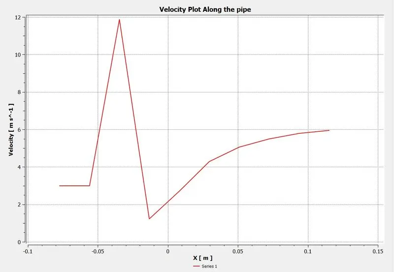
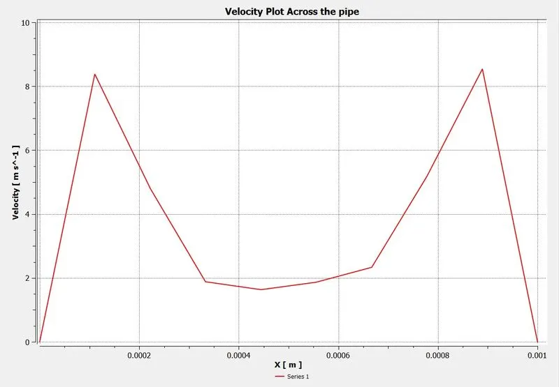
Fig(g): Velocity Plot Along the pipe. Fig(h): Velocity Plot Across the pipe.
//*****************************************************************************************************************************************************\\
3. K-Omega model of Momentum ratio-2.
MESHING:-
The model is meshed using ANSYS Mesher with the above element size. And give the named selection for inlet, outlet, and Walls.
Element size = 2 mm
Mesh Metric:
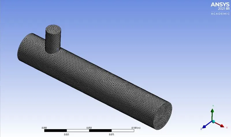
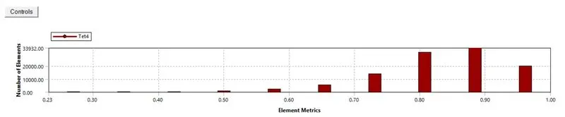
Element Quality:
- Minimum = 0.23159
- Maximum = 1
- Average = 0.83717
- Std.Deviation = 9.4e-2
SETUP FLUENT:-
From the setup to set the solver, turbulence model, and other physics.
Solver:
Type = Pressure based
Time = Steady
Velocity Formulation = Absolute
Viscous Model:
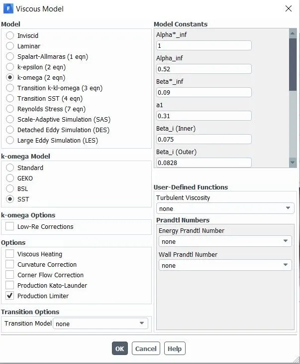
Boundaries:
1. Inlet x (Hot inlet)
Velocity Magnitude = 3 m/s.
Temperature = 36°C
2. Inlet y (cold inlet)
Velocity Magnitude = 6 m/s.
Temperature = 19°C
Report Definitions :
- Area-Weighted average of temperature
- Standard Deviation of temperature
Run the Calculation:
No. of Iteration = 400
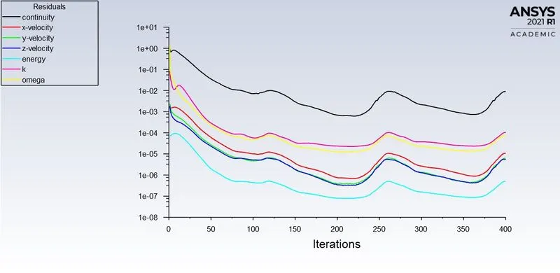
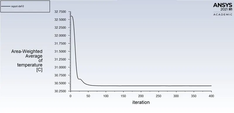
Fig(1): Residuals Plot Fig(2): Area-Weighted Average plot
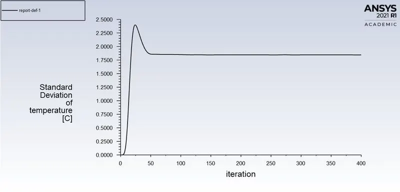
Fig(3): Standard Deviation Plot
From the graph,
- The flow is converged after 145 iterations.
- The Average Outlet temperature is 30.414824°C
- The Simulation time is 388.868 sec.
POST-PROCESSING RESULT:-
1. Temperature Contour plot on the cut planes along and across the pipe.
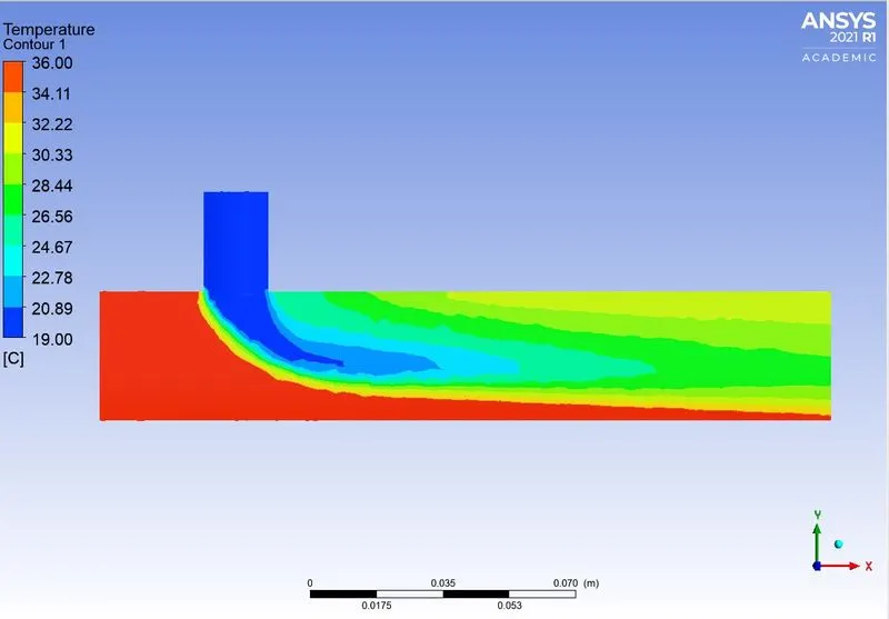
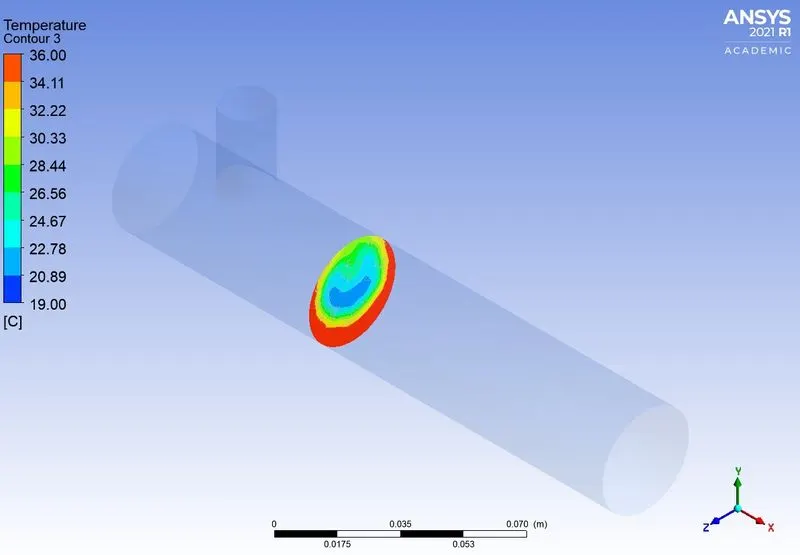
Fig(a): Temperature Contour Along the XY plane. Fig(b): Temperature Contour Across the YZ plane.
2. Velocity Contour plot on the cut planes along and across the pipe.
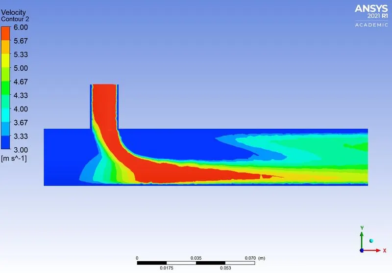
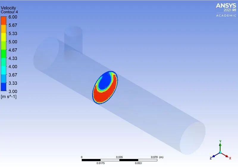
Fig(c): Velocity Contour along the XY plane. Fig(d): Velocity Contour Across the YZ plane.
3. Temperature line plot along and across the length of the pipe.
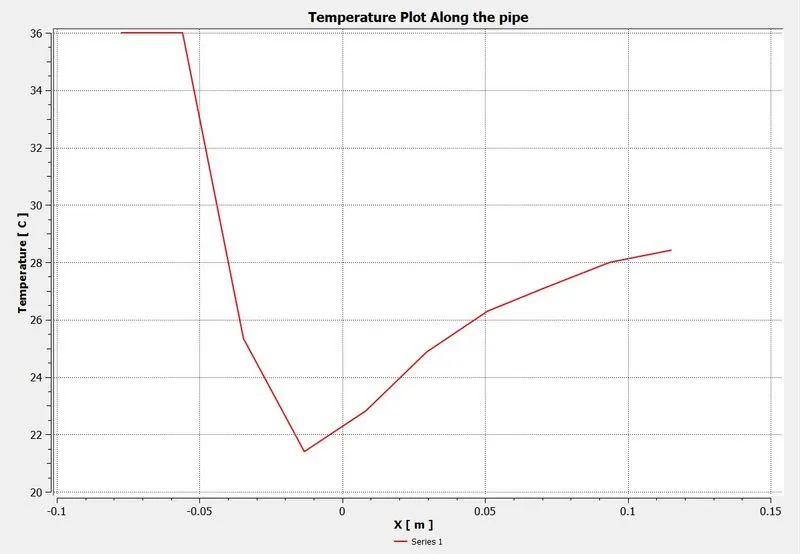
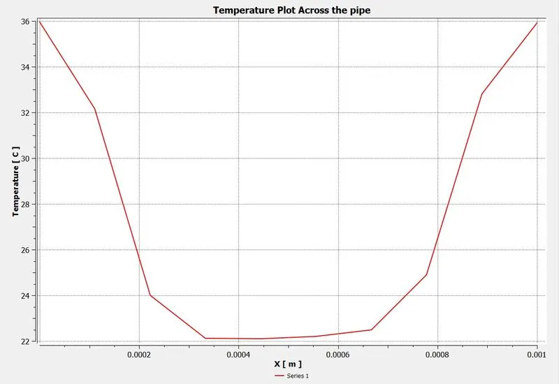
Fig(e): Temperature Plot Along the pipe. Fig(f): Temperature Plot Across the pipe.
4. Velocity line plot along and across the length of the pipe.
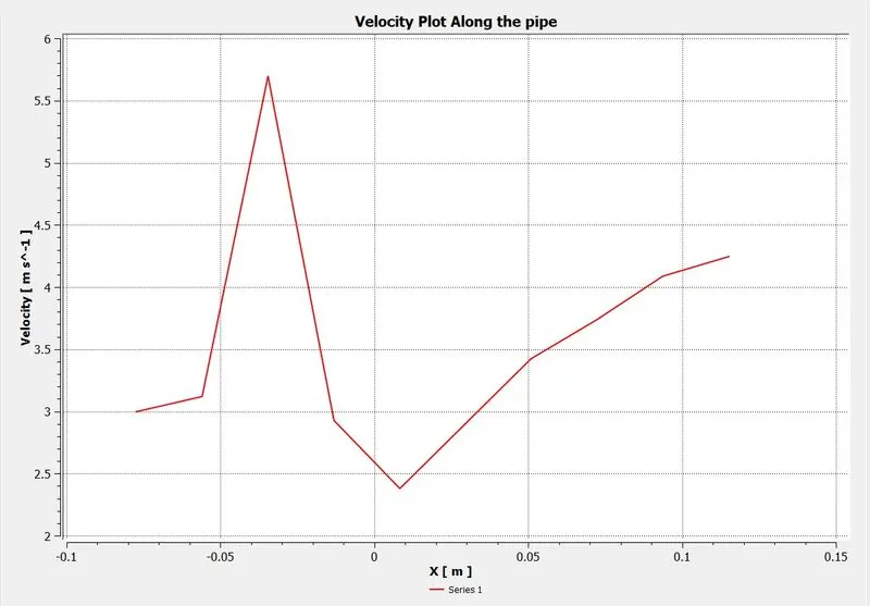
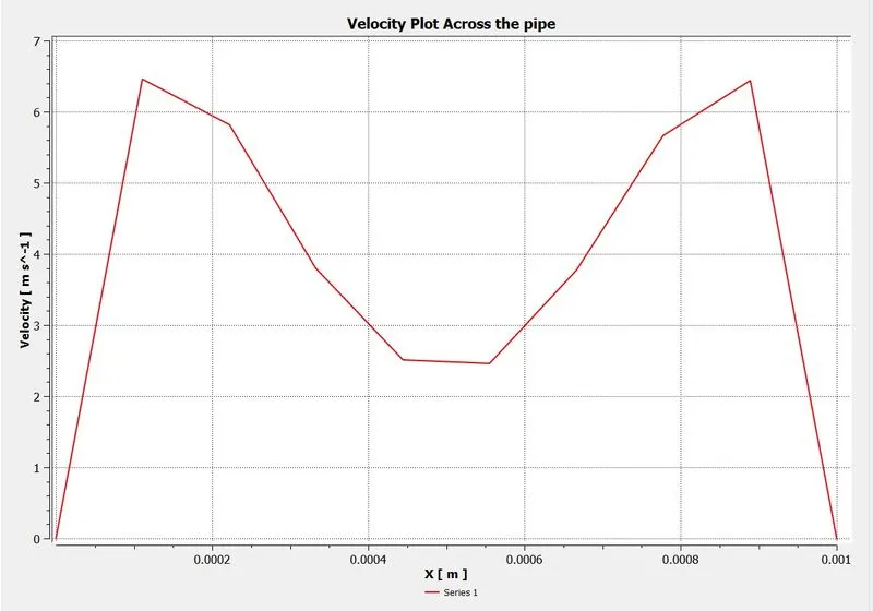
Fig(g): Velocity Plot Along the pipe. Fig(h): Velocity Plot Across the pipe.
//*****************************************************************************************************************************************************\\
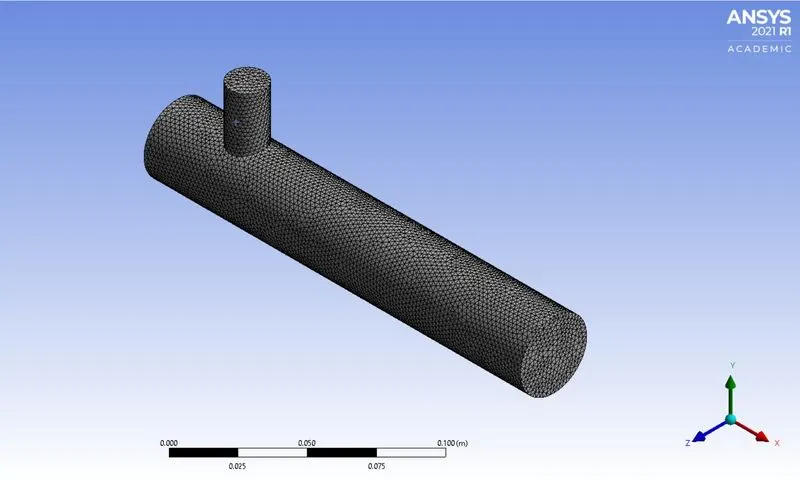
4. K-Omega model of Momentum ratio-4.
MESHING:-
The model is meshed using ANSYS Mesher with the above element size. And give the named selection for inlet, outlet, and Walls.
Element size = 2 mm
Mesh Metric:
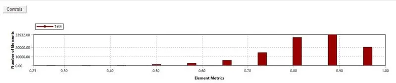
Element Quality:
- Minimum = 0.23159
- Maximum = 1
- Average = 0.83717
- Std.Deviation = 9.4e-2
SETUP FLUENT:-
From the setup to set the solver, turbulence model, and other physics.
Solver:
- Type = Pressure based
- Time = Steady
- Velocity Formulation = Absolute
Viscous Model:
Boundaries:
1. Inlet x (Hot inlet)
Velocity Magnitude = 3 m/s.
Temperature = 36°C
2. Inlet y (cold inlet)
Velocity Magnitude = 12 m/s.
Temperature = 19°C
Report Definitions :
- Area-Weighted average of temperature
- Standard Deviation of temperature
Run the Calculation:
No. of Iteration = 400
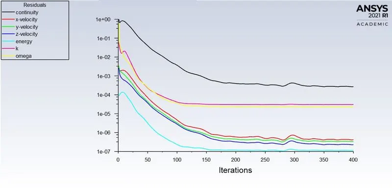
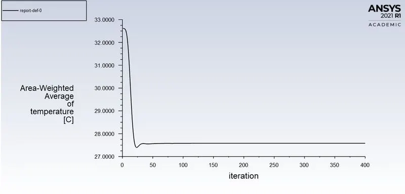
Fig(1): Residuals Plot Fig(2): Area-Weighted Average plot
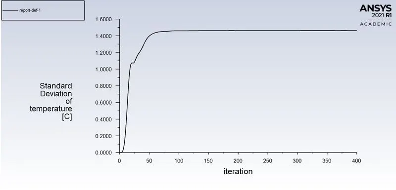
Fig(3): Standard Deviation Plot
From the graph,
- The flow is converged after 180 iterations.
- The Average Outlet temperature is 27.581786°C
- The Simulation time is 354.797 sec.
POST-PROCESSING RESULT:-
1. Temperature Contour plot on the cut planes along and across the pipe.
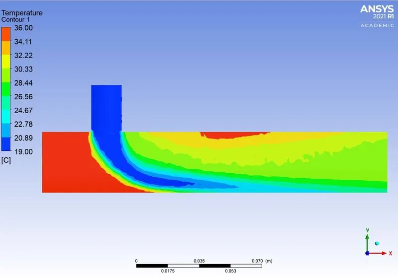
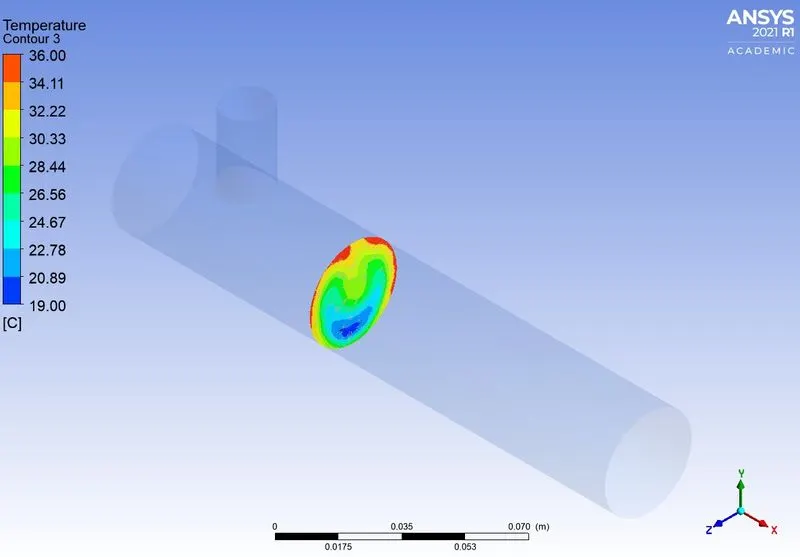
Fig(a): Temperature Contour Along the XY plane. Fig(b): Temperature Contour Across the YZ plane.
2. Velocity Contour plot on the cut planes along and across the pipe.
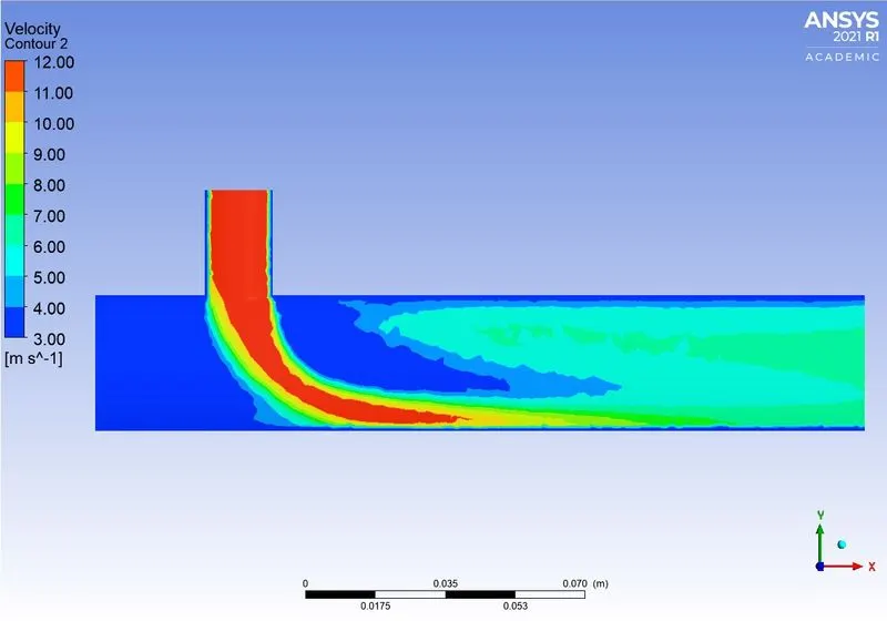
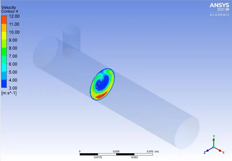
Fig(c): Velocity Contour along the XY plane. Fig(d): Velocity Contour Across the YZ plane.
3. Temperature line plot along and across the length of the pipe.
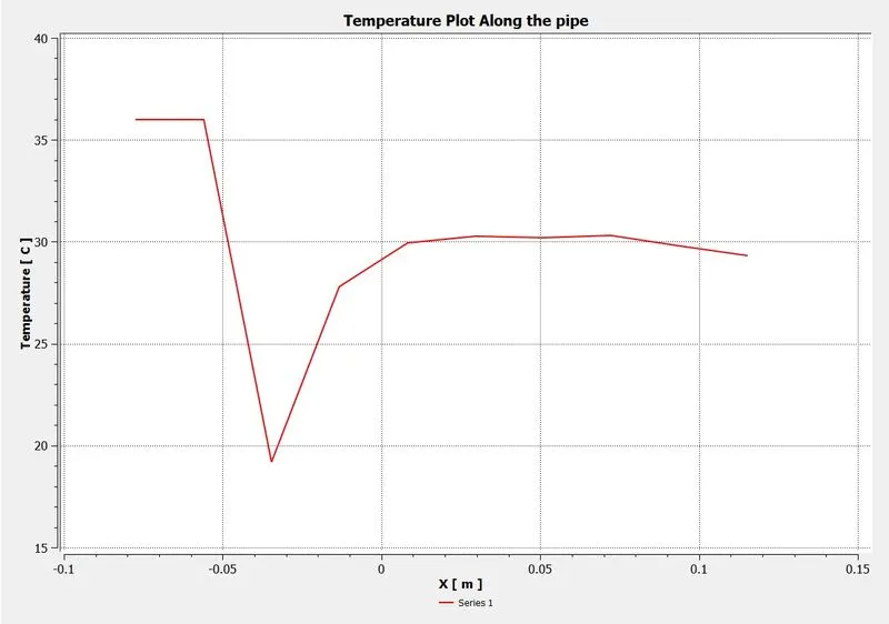
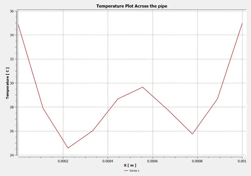
Fig(e): Temperature Plot Along the pipe. Fig(f): Temperature Plot Across the pipe.
4. Velocity line plot along and across the length of the pipe.
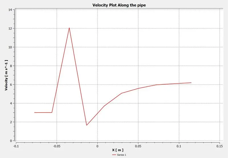
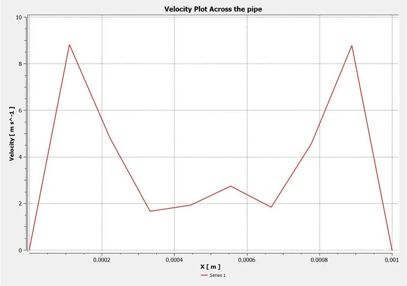
Fig(g): Velocity Plot Along the pipe. Fig(h): Velocity Plot Across the pipe.
//*****************************************************************************************************************************************************\\
CASE- 2 (LONG MIXING TEE):-
In this case, simulating the long mixing tee with the momentum ratio of 2 and 4. And the K - Epsilon Turbulence model is used.
- K-Epsilon model of Momentum ratio - 2
- K-Epsilon model of Momentum ratio - 4
GEOMETRY MODEL:-
Fig 1: The geometry of a Long mixing tee.
Volume Extract using SpaceClaim:
The flow volume is extracted from the geometry by SpaceClaim in ANSYS Fluent to measure the pipe's mixing effectiveness.
Fig 2: The volume extracted geometry.
1. K-Epsilon model of Momentum ratio-2.
MESHING:-
The model is meshed using ANSYS Mesher with the above element size. And give the named selection for inlet, outlet, and Walls.
Element size = 2 mm
Mesh Metric:
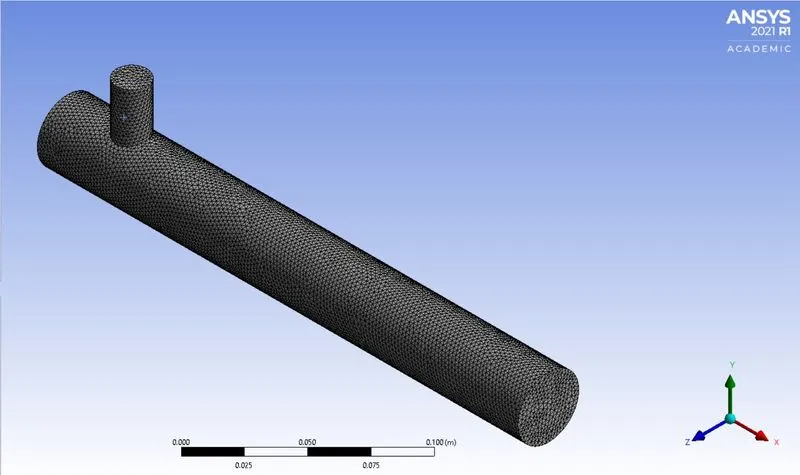
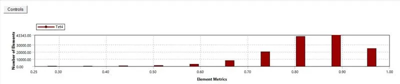
Element Quality:
- Minimum = 0.24801
- Maximum = 1
- Average = 0.8357
- Std.Deviation = 9.4E-2
SETUP FLUENT:-
From the setup to set the solver, turbulence model, and other physics.
Solver:
- Type = Pressure based
- Time = Steady
- Velocity Formulation = Absolute
Viscous Model:
Boundaries:
1. Inlet x (Hot inlet)
Velocity Magnitude = 3 m/s.
Temperature = 36°C
2. Inlet y (cold inlet)
Velocity Magnitude = 6 m/s.
Temperature = 19°C
Report Definitions :
- Area-Weighted average of temperature
- Standard Deviation of temperature
Run the Calculation:
No. of Iteration = 400
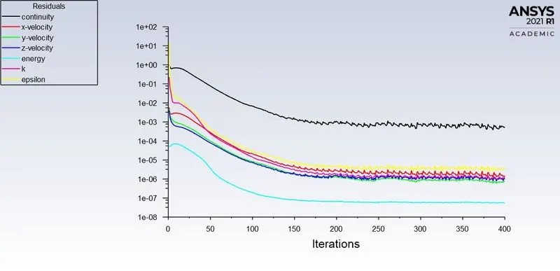
Fig(1): Residuals Plot Fig(2): Area-Weighted Average plot
Fig(3): Standard Deviation Plot
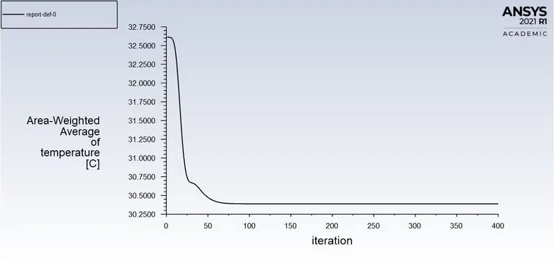
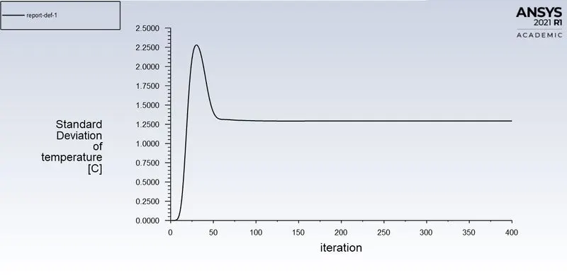
From the graph,
- The flow is converged after 140 iterations.
- The Average Outlet temperature is 30.387878°C
- The Simulation time is 626.9715 sec.
POST-PROCESSING RESULT:-
1. Temperature Contour plot on the cut planes along and across the pipe.
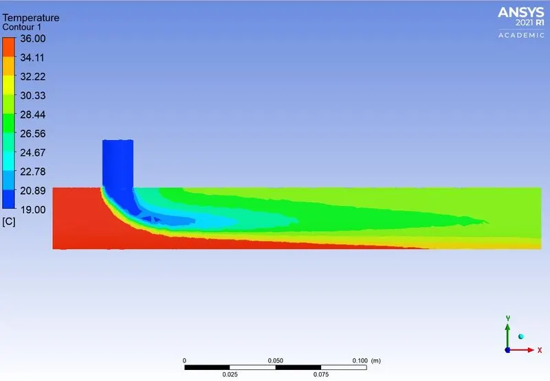
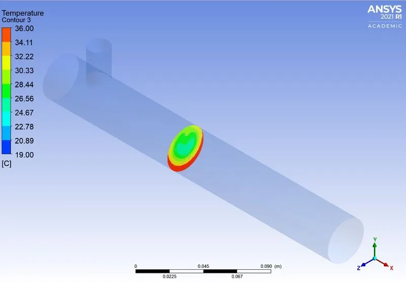
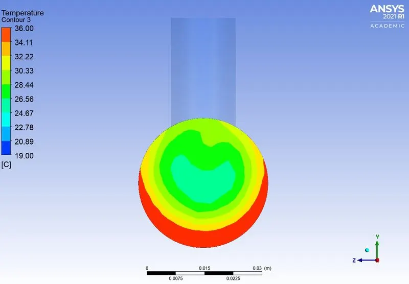
Fig(a): Temperature Contour Along the XY plane. Fig(b): Temperature Contour Across the YZ plane.
2. Velocity Contour plot on the cut planes along and across the pipe.
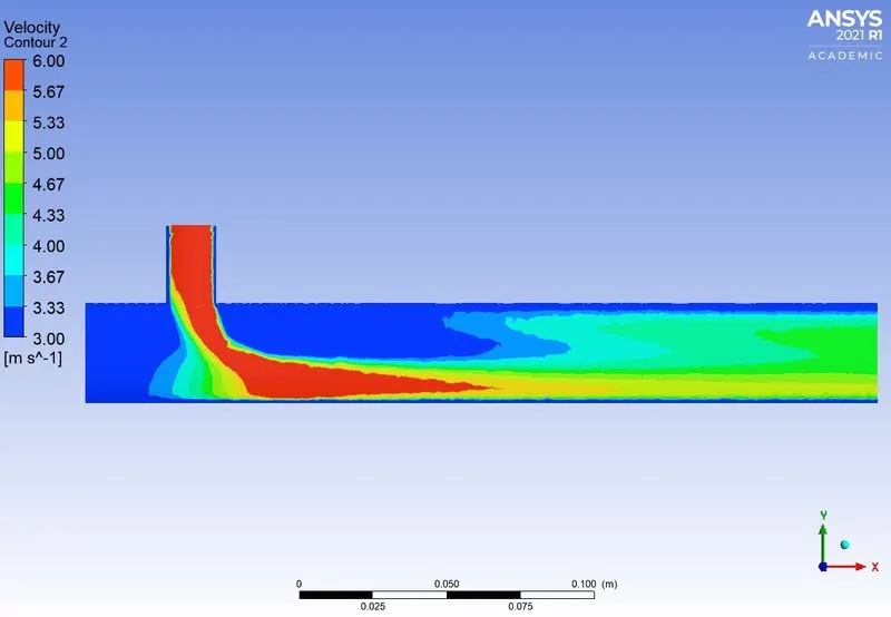
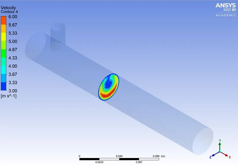
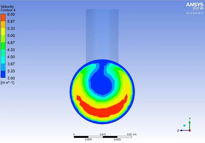
Fig(c): Velocity Contour along the XY plane. Fig(d): Velocity Contour Across the YZ plane.
3. Temperature line plot along and across the length of the pipe.
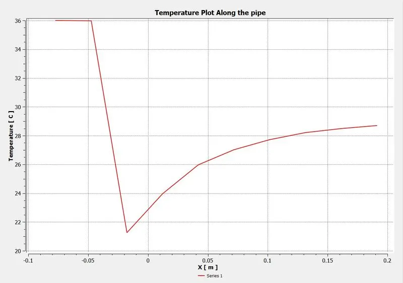
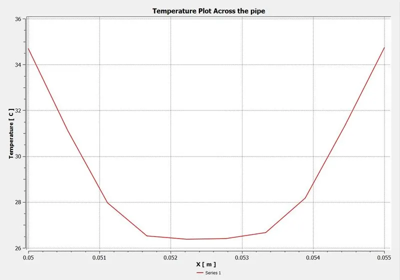
Fig(e): Temperature Plot Along the pipe. Fig(f): Temperature Plot Across the pipe.
4. Velocity line plot along and across the length of the pipe.
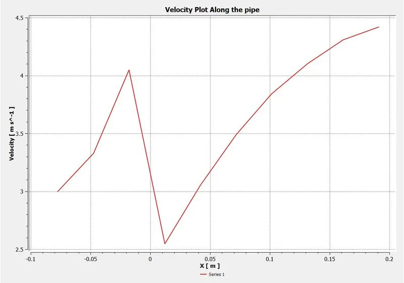
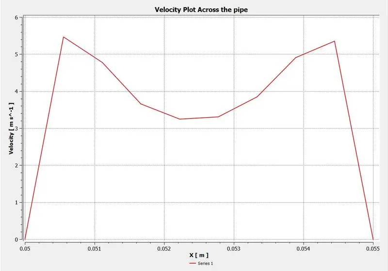
Fig(g): Velocity Plot Along the pipe. Fig(h): Velocity Plot Across the pipe.
//*****************************************************************************************************************************************************\\
2. K-Epsilon model of Momentum ratio - 4.
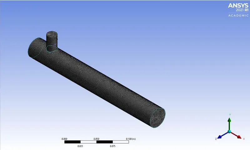
MESHING:-
The model is meshed using ANSYS Mesher with the above element size. And give the named selection for inlet, outlet, and Walls.
Element size = 2 mm
Mesh Metric:
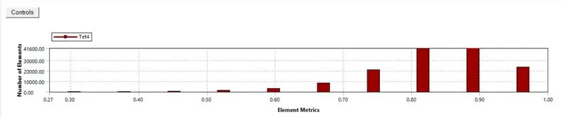
Element Quality:
- Minimum = 0.2684
- Maximum = 1
- Average = 0.83578
- Std.Deviation = 9.39e-2
SETUP FLUENT:-
From the setup to set the solver, turbulence model, and other physics.
Solver:
- Type = Pressure based
- Time = Steady
- Velocity Formulation = Absolute
Viscous Model:
Boundaries:
1. Inlet x (Hot inlet)
Velocity Magnitude = 3 m/s.
Temperature = 36°C
2. Inlet y (cold inlet)
Velocity Magnitude = 12 m/s.
Temperature = 19°C
Report Definitions :
- Area-Weighted average of temperature
- Standard Deviation of temperature
Run the Calculation:
No. of Iteration = 400
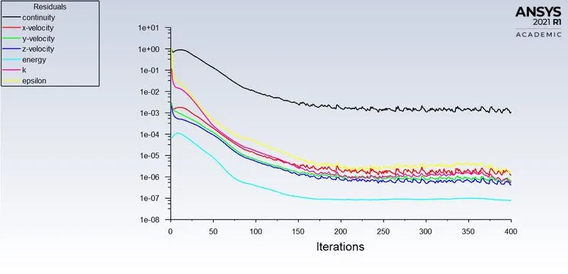
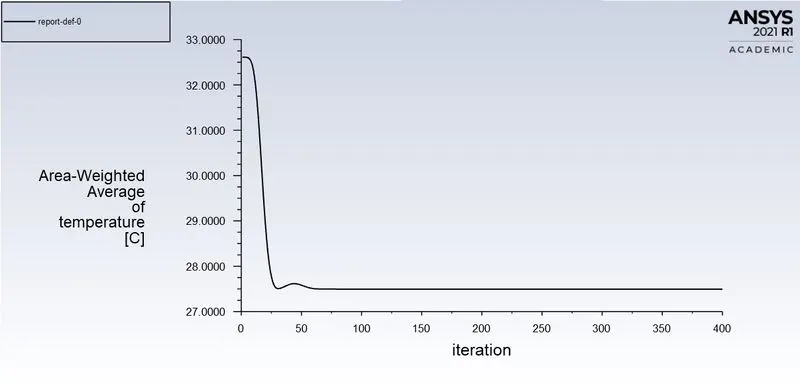
Fig(1): Residuals Plot Fig(2): Area-Weighted Average plot
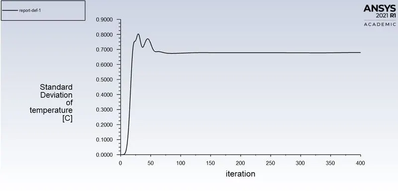
Fig(3): Standard Deviation Plot
From the graph,
- The flow is converged after 175 iterations.
- The Average Outlet temperature is 27.495548°C
- The Simulation time is 769.444 sec.
POST-PROCESSING RESULT:-
1. Temperature Contour plot on the cut planes along and across the pipe.
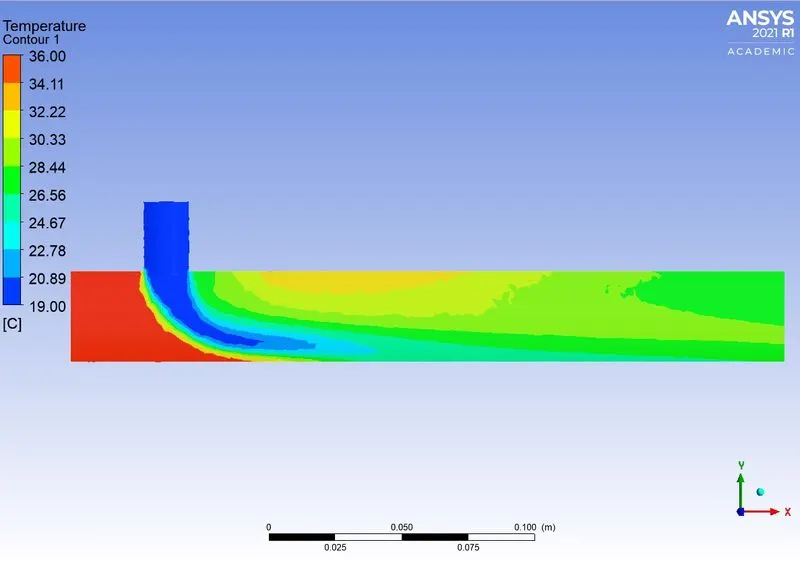
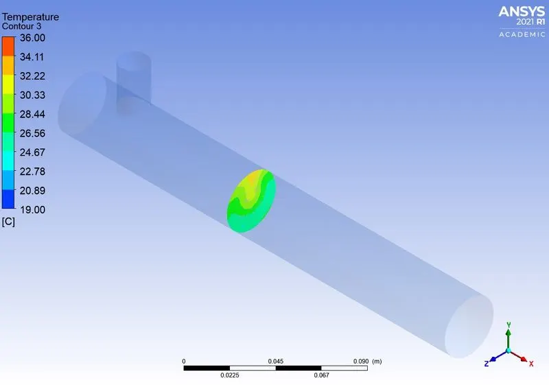
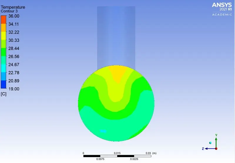
Fig(a): Temperature Contour Along the XY plane. Fig(b): Temperature Contour Across the YZ plane.
2. Velocity Contour plot on the cut planes along and across the pipe.
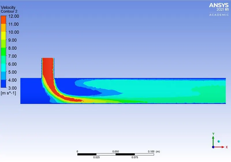
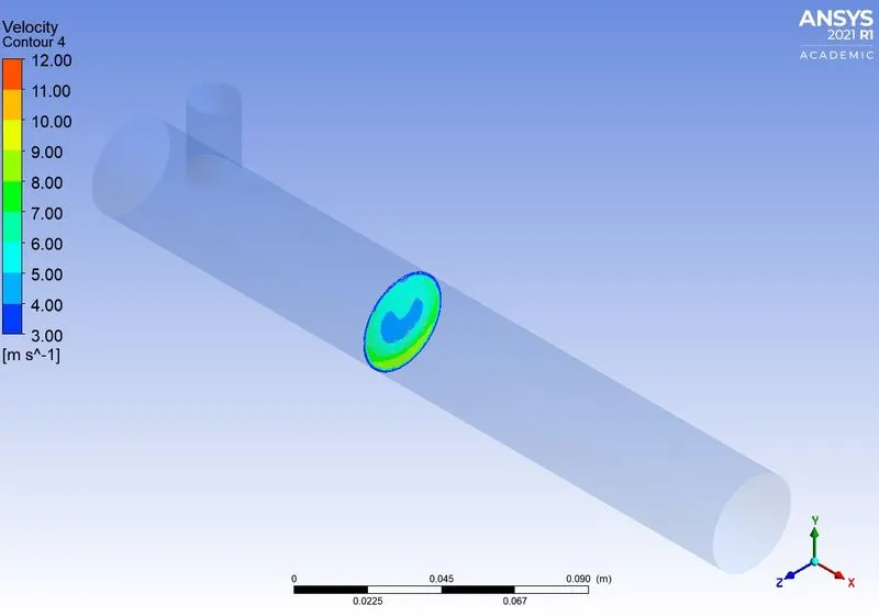
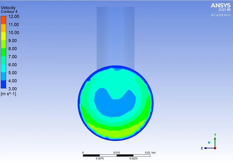
Fig(c): Velocity Contour along the XY plane. Fig(d): Velocity Contour Across the YZ plane.
3. Temperature line plot along and across the length of the pipe.
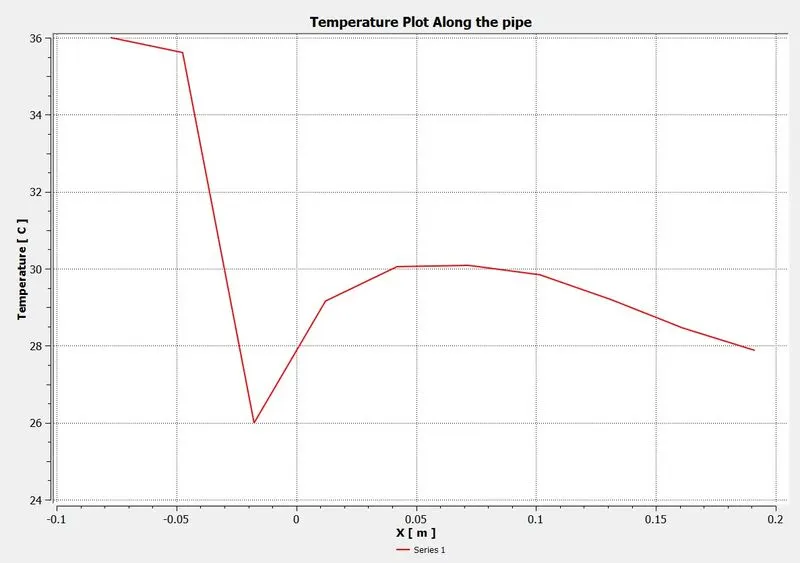
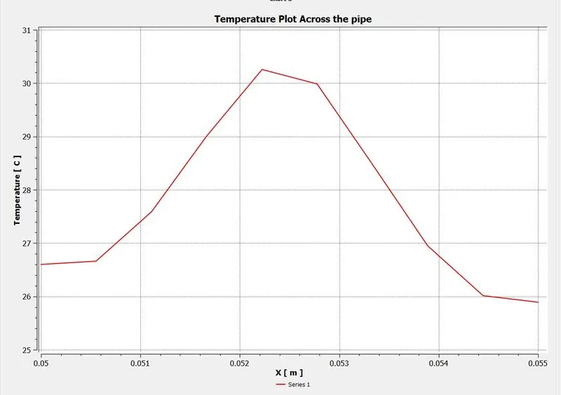
Fig(e): Temperature Plot Along the pipe. Fig(f): Temperature Plot Across the pipe.
4. Velocity line plot along and across the length of the pipe.
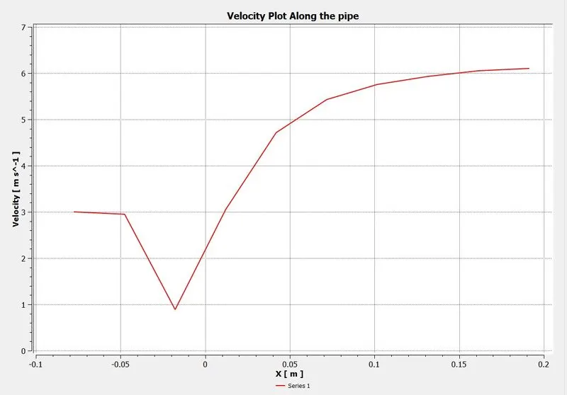
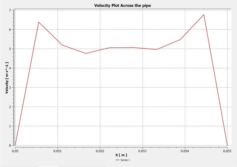
Fig(g): Velocity Plot Along the pipe. Fig(h): Velocity Plot Across the pipe.
//*****************************************************************************************************************************************************
Tabulation:-
Case Model Cell Count Avg. Outlet Temperature No. of Iteration for convergence Simulation time
1. K-Epsilon model of M.R - 2 105858 30.299281 120 343.456
K-Epsilon model of M.R - 4 105858 27.586247 155 353.377
K-Omega model of M.R - 2 105858 30.414824 145 388.868
K-Omega model of M.R - 4 105858 27. 581786 180 354.797
2. K-Epsilon model of M.R - 2 140025 30.387878 140 626.9715
K-Epsilon model of M.R - 4 140025 27.495548 175 769.444
Conclusion:-
Case 1 (Short Mixing Tee):
- The Avg. outlet temp of the K-epsilon model of momentum ratio - 2 (which means cold velocity is 6 m/s) is 30.299281
- The Avg. outlet temp of the K-epsilon model of momentum ratio - 4 (which means cold velocity is 12m/s) is 27.586247
Case 2 (Long Mixing Tee):
- The Avg. outlet temp of the K-epsilon model of momentum ratio - 2 (which means cold velocity is 6 m/s) is 30.387878
- The Avg. outlet temp of the K-epsilon model of momentum ratio - 4 (which means cold velocity is 12m/s) is 27.495548
- By comparing the case 1 & 2 there is no difference between the outlet temperature. so, the change in length of the pipe should not affect the mixing of the flow.
- If the velocity increase(Momentum ratio) the temperature is reduced.
- And the K - Epsilon turbulence model simulation is faster than the K - Omega model.
- From the above tabulation and post-processing result, we can say if the velocity increases the outlet temperature should be decreased.
Effects of Length:
The Change in length of the pipe should not change the outlet temperature. Only the number of elements and simulation time should be increased.
Momentum Ratio:
The momentum ratio is inversely proportional to the Average outlet temperature. If the momentum ratio (cold inlet velocity) increases the average outlet temperature is decreased.