Week 1- Mixing Tee

Aim:-

• Set up steady-state simulations to compare the mixing effectiveness when the hot inlet temperature is 36C, and the cold inlet is 19C.
• Try both the k-epsilon and k-omega SST models for the first case to get proper judgment about each method; later, use the most suitable model for further simulations.
• Simulate each case for the given velocity and momentum ratio.
• Compare results from the 2 cases about cell count, average outlet temperature, and the number of iterations for convergence.
• Plot the velocity and temperature contour plots on the cut plane along and across the pipe.
• Also, plot the velocity and temperature line plots along and across the length of the pipe.
• Perform Mesh independent study for any one case.
• Moreover, discuss the effect of length and momentum ratio on results.
• Lastly, for each simulation, show the convergence plot.

Objective:-

• Understand and define the problem statement for each case.
• Open Ansys workbench and set up a fluent simulation setup, and rename it accordingly.
• From fluent setup, open space claims, and Load the geometry. Extract the working fluid region from the loaded geometry to compute simulation in that particular region. And then close space claim.
• Next, in mesh setup, provide boundary names for each surface and generate mesh to the fluid flow volume. Close mesh setup and update the mesh.
• Later, in the setup section, provide all the required parameters according to the simulation, such as simulation type, input velocity and temperature, materials (working fluid), and other user-defined parameters.
• In setup parameters, understand the concept of k-epsilon and k-omega SST and find out which is convenient for the current simulation.
• Afterward, simulate our problem setup for the number of iteration required to converge our results.
• Then, close and update the setup. Open the results section to see all the simulated results.
• Juxtapose generated results from each case for their cell count, average outlet temperature, and the number of iteration for convergence.
• Display contour plot on the cut plane to visualize velocity and temperature distribution along and across the mixing tee’s length.
• For a more detailed examination, plot velocity and temperature line chart along the mixing tee’s length.
• Validate the test by performing a mesh independence study on any one case.
• Study the effect of length and momentum ratio on the results of each case.
• Plot the convergence graph to verify that all the results are fully converged after running numerous iterations.

Problem Setup

Understand k-epsilon and k-omega SST by considering case-1

Case-1

Short mixing tee

a - Simulation-1

hot Inlet velocity - 3m/s

Momentum ratio - 2

b - Simulation-2

hot Inlet velocity - 3m/s

Momentum ratio - 4

A] K-epsilon:-

Now for the simulation-1, We are considering the movement ratio of 2 m/s at Cold air inlet. We have selected K-epsilon model for the simulation. Lets look at the following results from the simulations:-

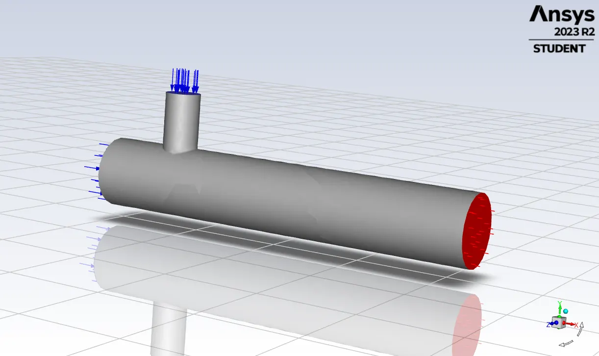
We have Provide the Inlet-X for the hot air at 32 degree C and Velocity of 3m/s. In the Inlet-y Direction we have set the value for the cold air at 19 degree C and velocity of 2 m/s. Some consideration are taken into the account before plotting the results.

1. We are using Energy equations because its involve temperature base calculations at outlet.

2. We are using pressure-based solver because the fluid flows with small density variation means its has very low mach number (u/v) where compressibility effects are negligible. The Pressure based solver works by coupling the velocity and pressure together, solving for the velocity first and then correcting the pressure.

3.We are using K-epsilon model with Realizable model. This Model is enhanced version of standard K-epsilon model. This model ensure that the certain mathematical and physical constrained are satisficed (like Kinetic Energy and Reynold stress)

4.For the Near-Wall Treatment we are using Standard Wall Function. They provide a flow properties such as velocity, temperature and turbulences without resolving very fine details at boundary layers.

Based on above setting we are plotting the graphs for Residuals, Area-Weighted Average for Temperature and Standard Deviations.

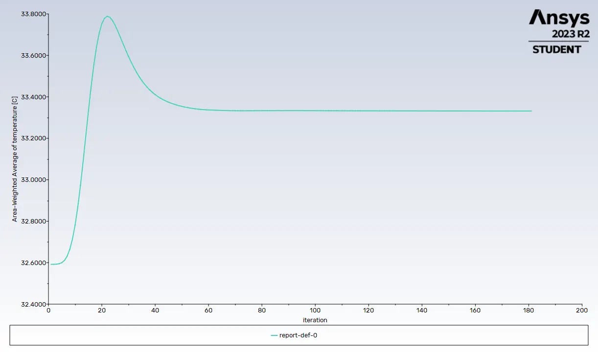
This graph is plotted against the Area-Weighted Average of Temperature. Now at 180th iterations the average temperature at different areas are 33.3 degree c. Now we look for standard deviation graph:-

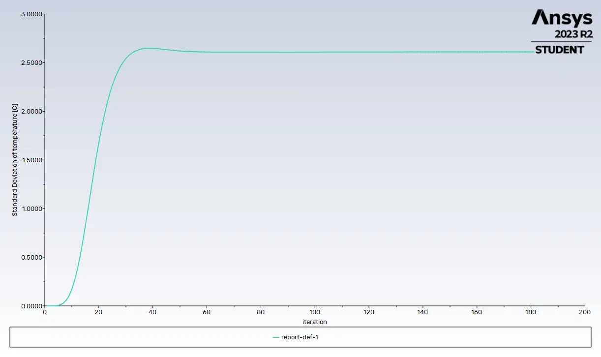
We can observed that the Standard Deviation of Temperature is 2.6 degree C. By comparing both results we can estimate that the temperature at outlet of pipe can be between 30.7 degree C to 35.9 degree C.

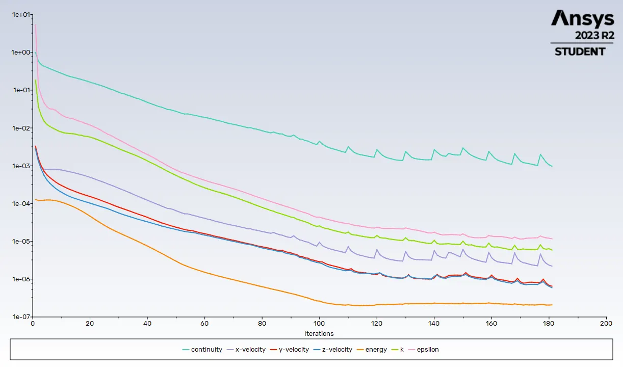
Now we look for the Scaled Residuals to analyze the conversion of each variables (continuity, velocity, energy ,k, epsilon). Scaled Residuals are a basically the difference between the computed solution and the actual solution .Its is the difference between left side and right side of the governing equation at each iteration. As the computed solution gets close or equal to actual solution, we achieved the steady state.

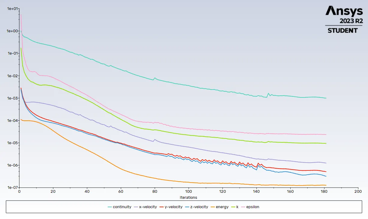
For the above graph we can estimate that at 180th iteration the difference between computed solution and actual solution is close to/equal to zero, that's where we achieve the steady state and our solution is converged can analyze the conversion rate for each variable with respect to iteration which helps us to know which variable are taking longer to convert or which variable caused the slow convergent rate.

Now we are plotting the result of our simulation. As per our estimation from graph we can observed that the temperature at outlet is between 30.7 degree C to 35.9 degree C.

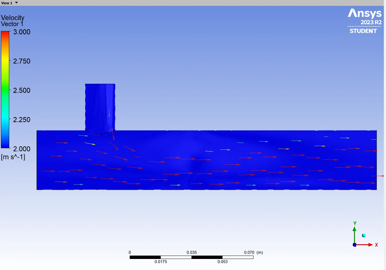
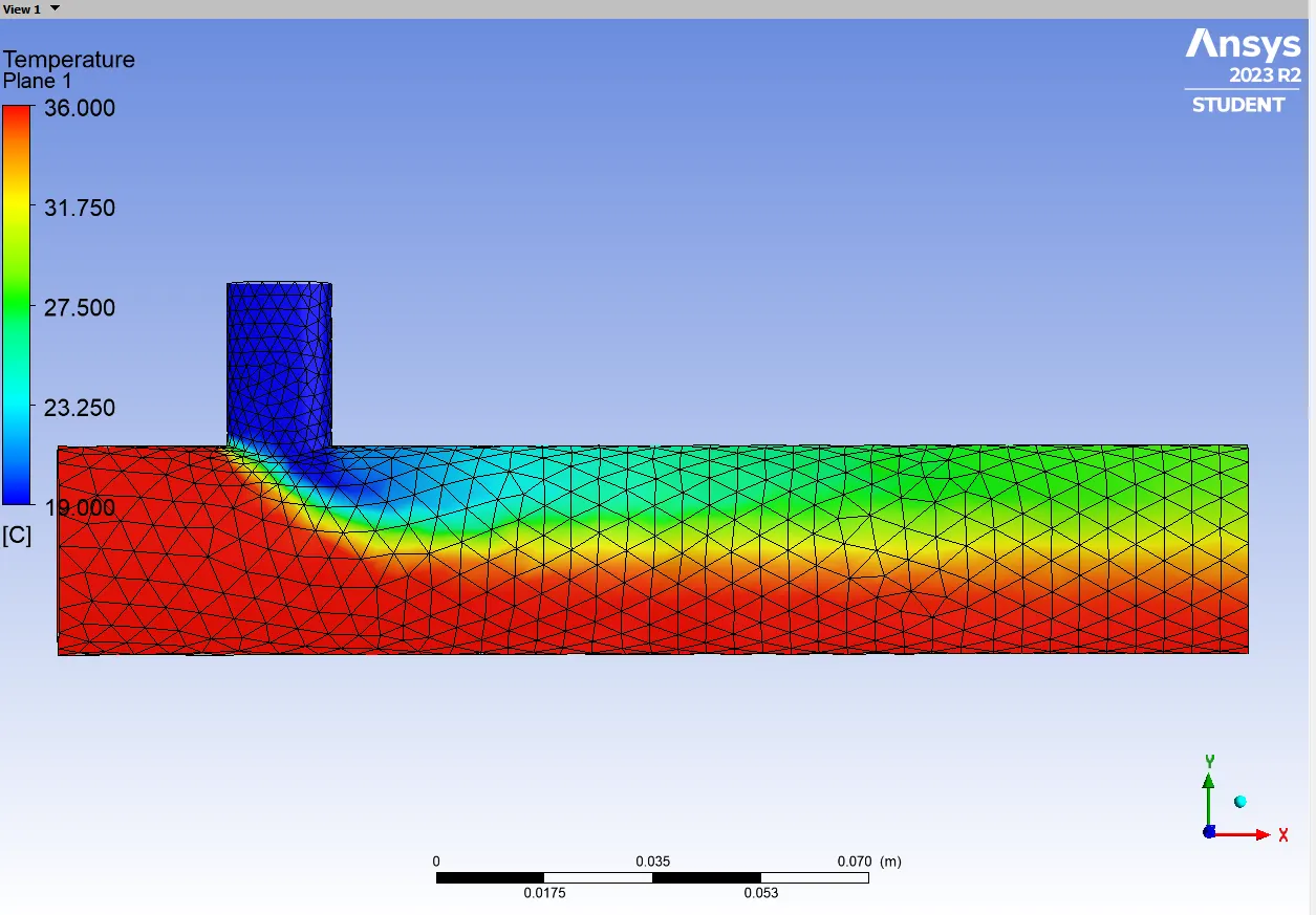
Now we are using the same module but for the different momentum ration of 4 m/s at inlet-y. Lets observe the result.

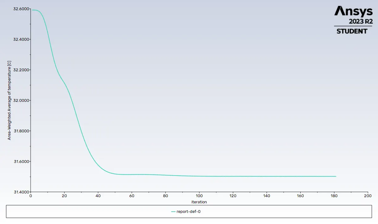
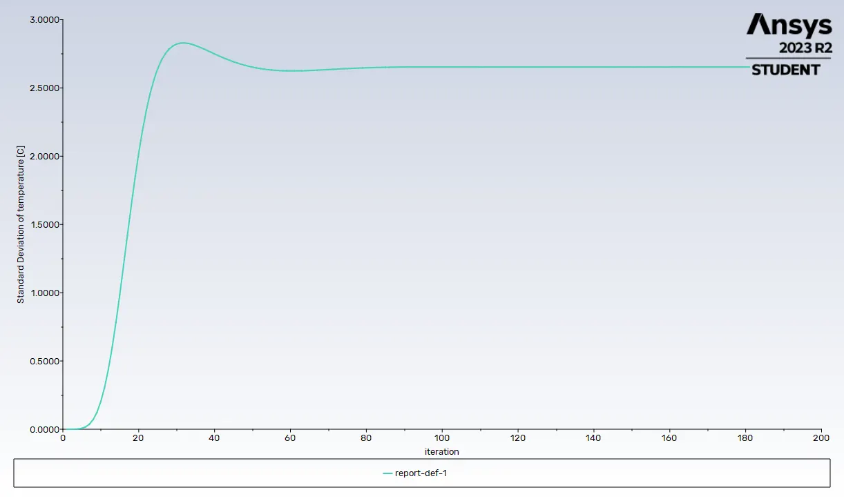
Based on above graph we can exanimate that the temperature at outlet will be between 28.9 degree C to 34.1 degree C.

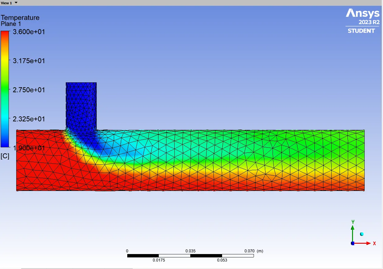
From above we can observed that the temperature at outlet as per the graph of standard deviation and area weighted average of temperature.

B] K-Omega SST:-

The K-omega model is used in CFD for simulating turbulent flow. It predict the turbulence by solving two transport equations one for the kinetic energy and another one for specific dissipation rate(Rate at which kinetic energy change into heat due to viscous fluid). This model works good for boundary conditions where turbulent, provide better efficiency near the wall. Turbulent kinetic energy(K) represent the energy contains in the turbulent Eddie. Omega describes the dissipation rate.

SST (Share Stress Transport):- SST uses both K-omega and K-epsilon that's why its called share stress Transport. It uses K-omega at boundary near the wall and its transform into K-epsilon when its away from the wall.

Production Limiter:- Production Limiter are used to limit the production of turbulent kinetic energy. It becomes too large in certain reigns.

Mow we are sing our first case with K-omega. Hot inlet will be 3m/s and cold inlet will be 2 m/s.

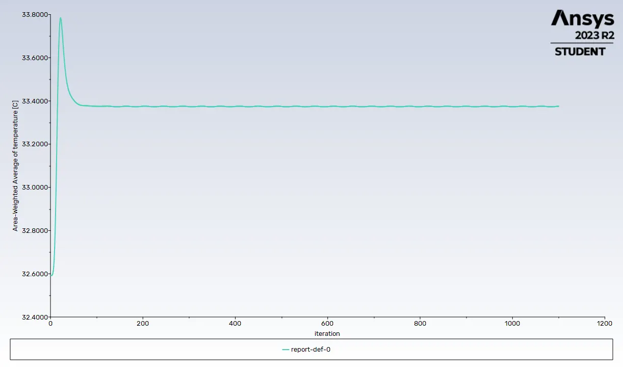
We we can see the Area-weighted Average of temperature graphs but we can see that its never reaches the steady state.

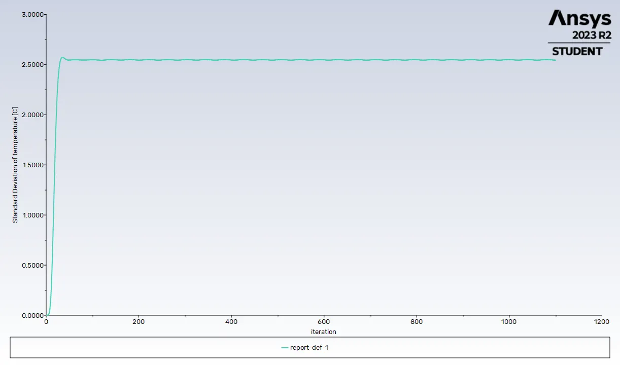
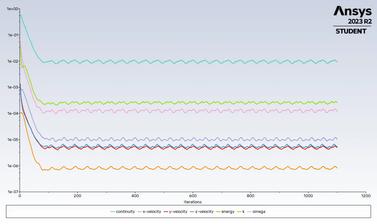
From Residual graph we can observe that the difference between computed value and actual value are not achieving equality. Its not just a one variable, we can also observed it for all variables. Lets see the post processing results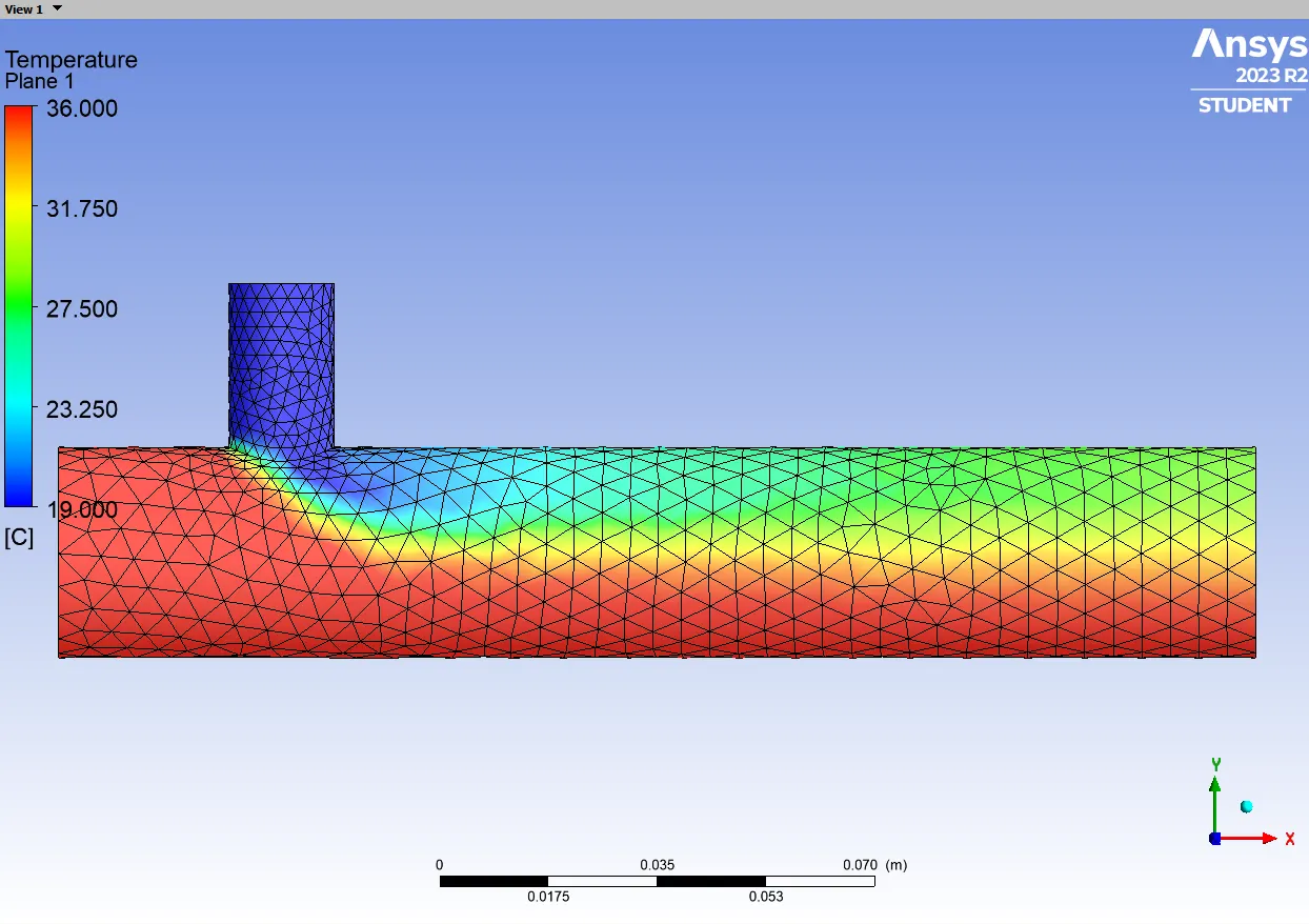

Lets applies the mesh independent study, We reduce the mesh size up to 0.001 , now we plot the result and observed if its archived steady state.

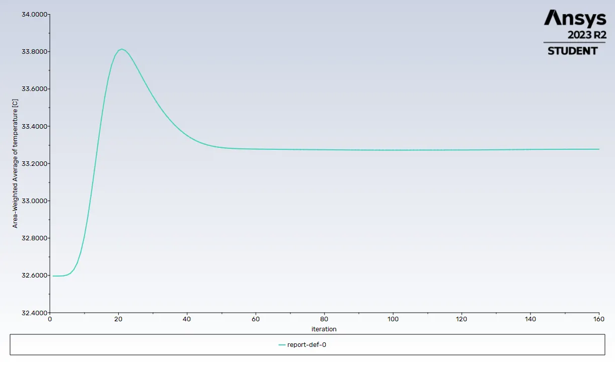
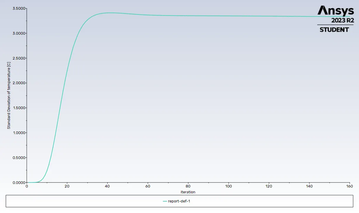
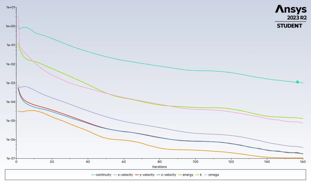
AT 160th iteration we have archived the steady state. Now from above graphs we can estimates the temperature between (32.27 + 3.38, 32.27-3.38) degree C

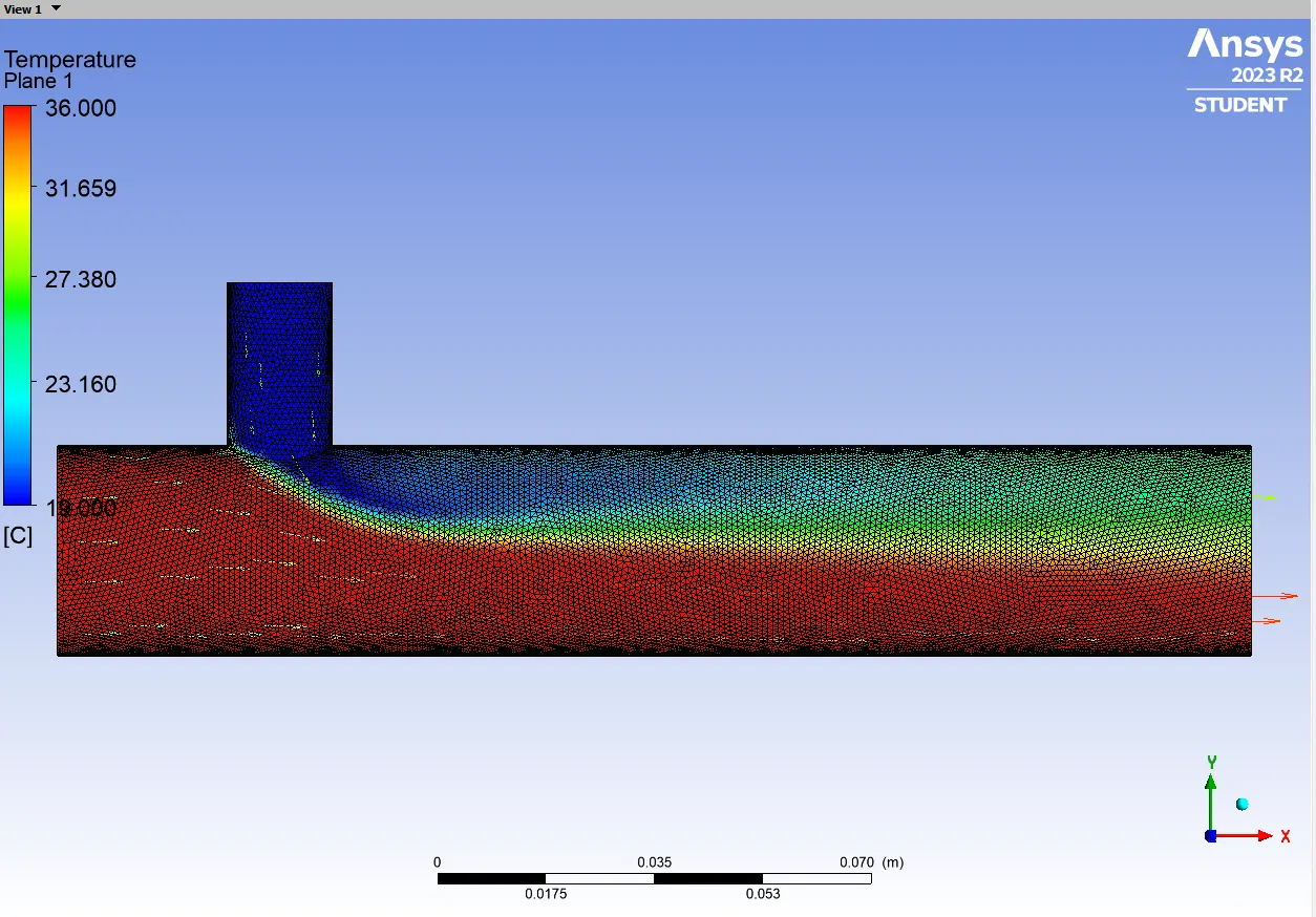
After performing the mesh independent study we reduce the mesh size that helps us to archive a smooth steady state transition.

Now we are using the same module but for the different momentum ration of 4 m/s at inlet-y. Lets observe the result.

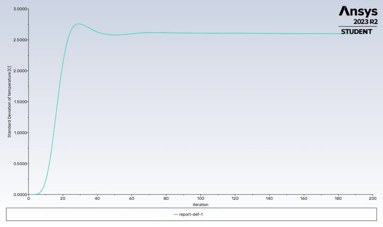
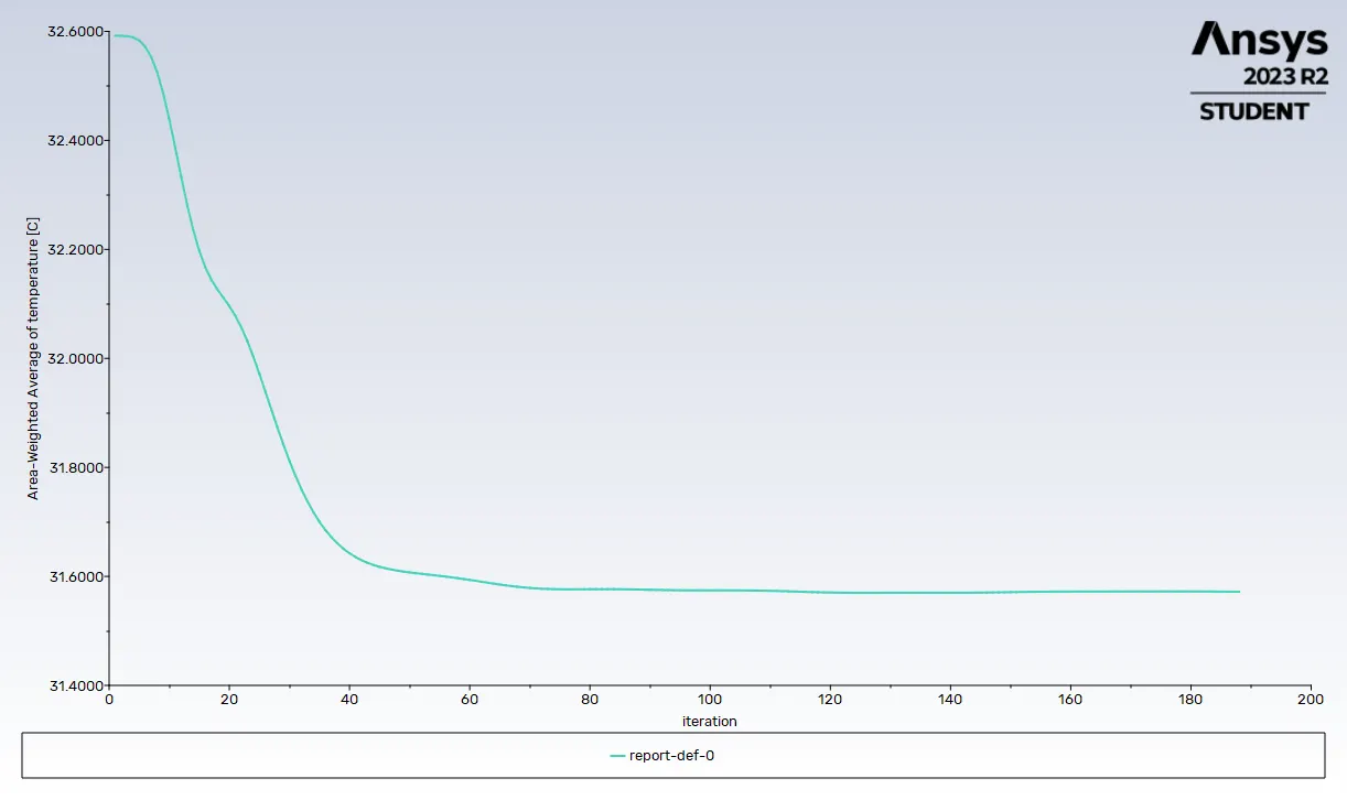
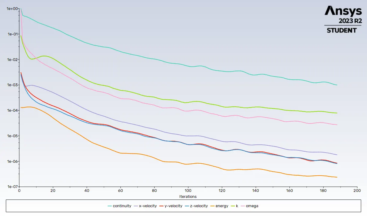
From Above graph we can estimate the temperature at outlet will be between 27.5 to 33.5 degree C.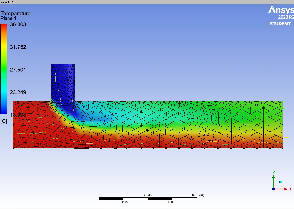

Main difference

The k- omega model is well suited for simulating flow in the viscous sub-layer. On the contrary, The k-epsilon model is ideal for predicting flow in the regions away from the wall

The SST model exhibit less sensitivity to free stream conditions (Flow outside the boundary layer) than many other turbulence models.

The shear stress limiter helps the k-omega model avoid a build-up of excessive turbulent kinetic energy near stagnation points.

If we observe our simulated figure, we can notice, in the k-omega model flow is more like laminar and not giving proper turbulent results, in contrast, simulation by k-epsilon, is giving proper mixing of the two air stream.

In this particular case we are not dealing with walls, therefore, we are going to use the k-epsilon method for further simulations.

In this particular case we are not dealing with walls, therefore, we are going to use the k-epsilon method for further simulations.

Now, let us start our simulation with case 1 -a

Case-2

Long mixing tee

a - Simulation-3

hot Inlet velocity - 3m/s

Momentum ratio - 2

b - Simulation-4

hot Inlet velocity - 3m/s

Momentum ratio - 4

In this case we are suing linger tee and analysis the effect on temperature if pipe length tee is increases.

Simulation-3:-

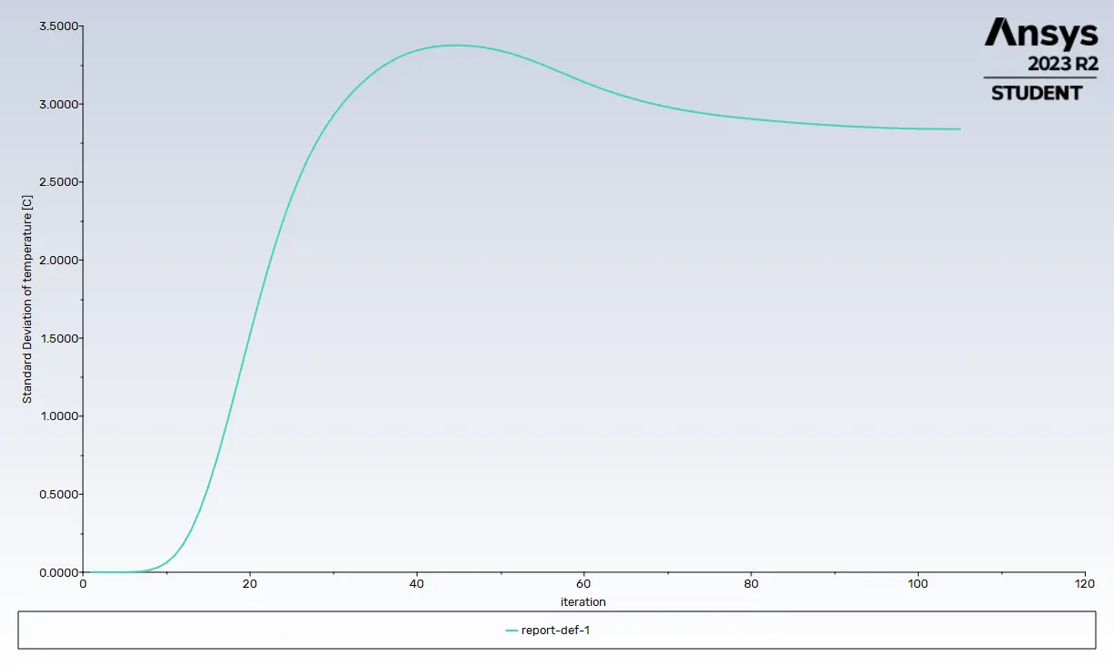
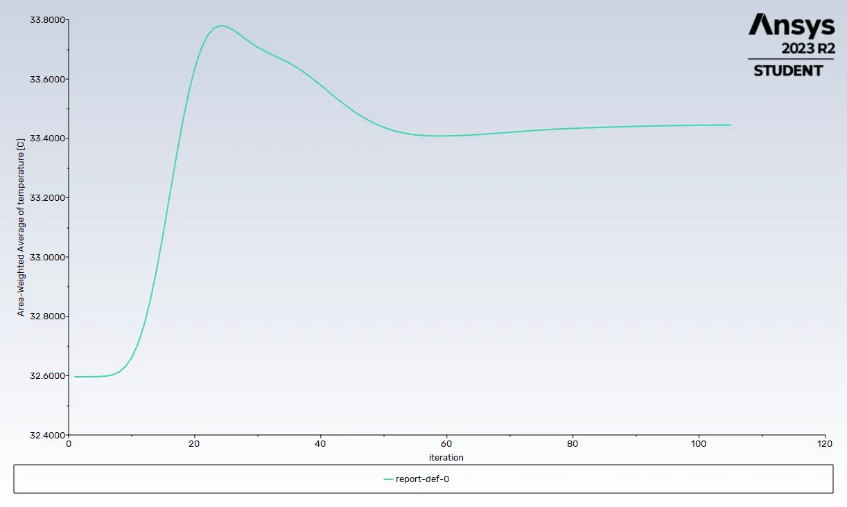
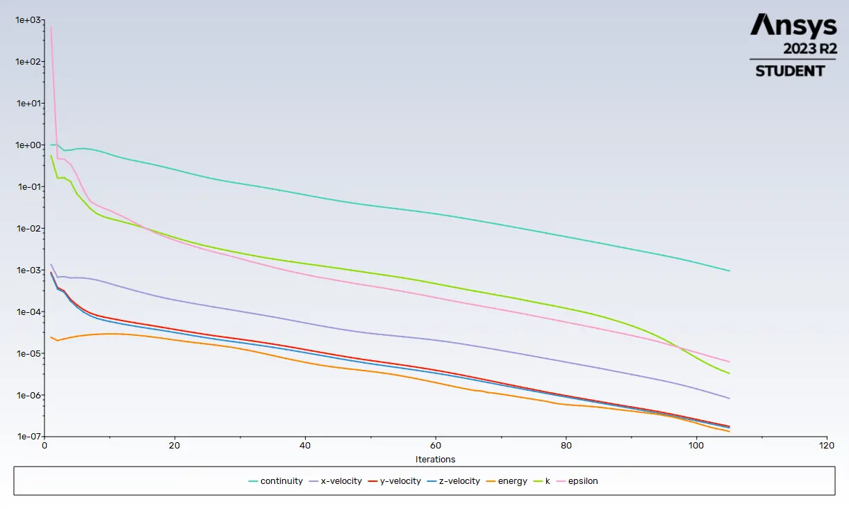
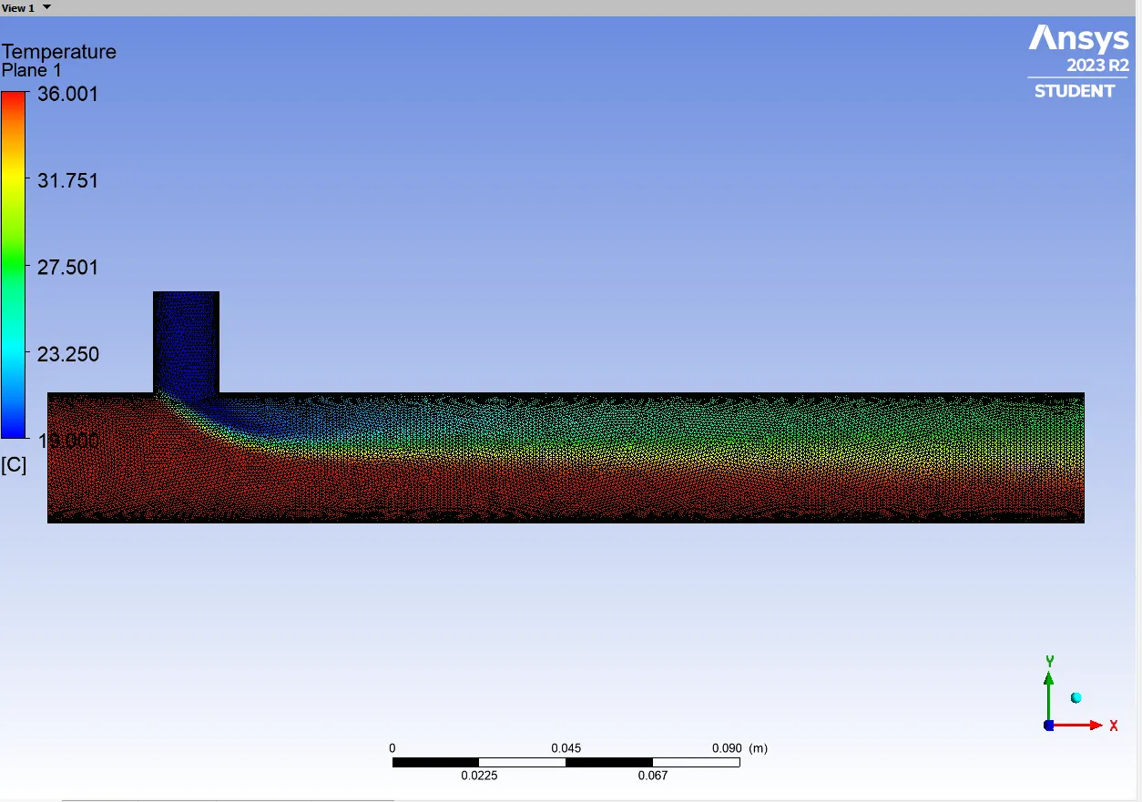
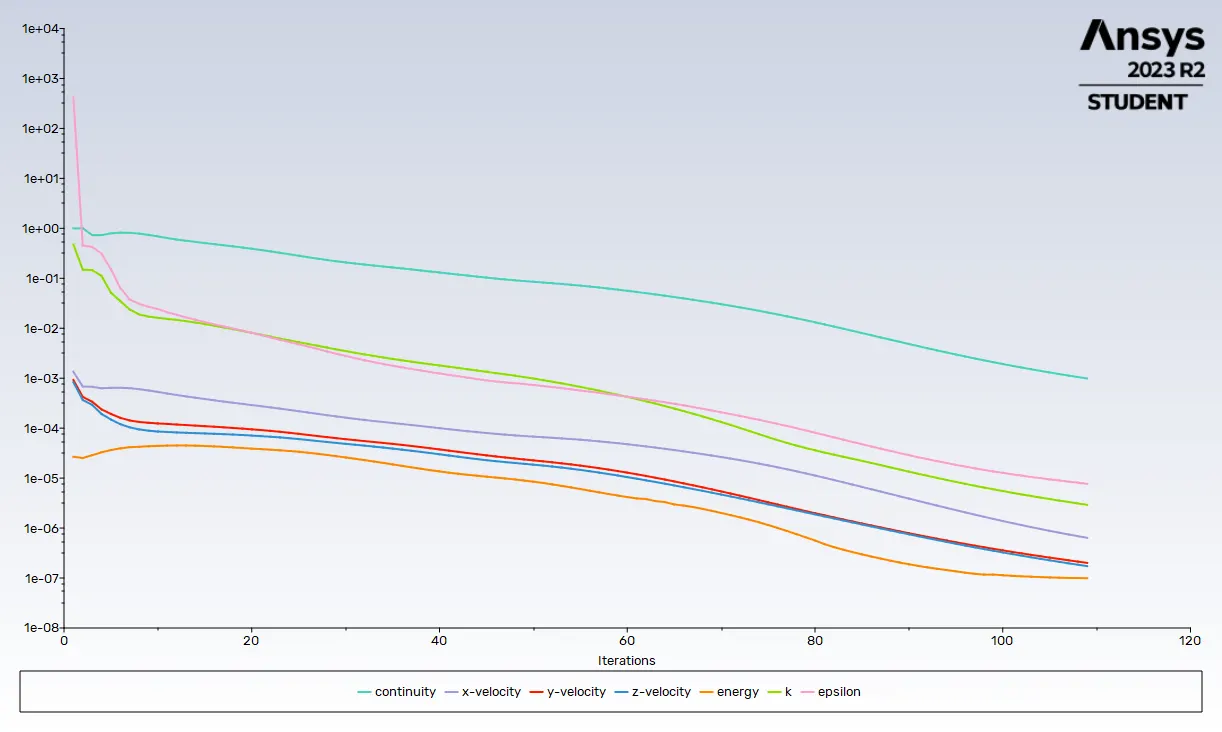
At 106th iteration, we achieved the steady state.

Now we perform the same set of equations for the 4m/s

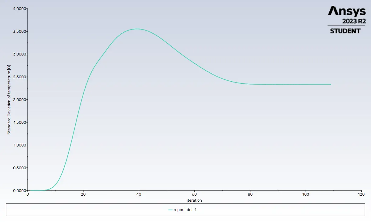
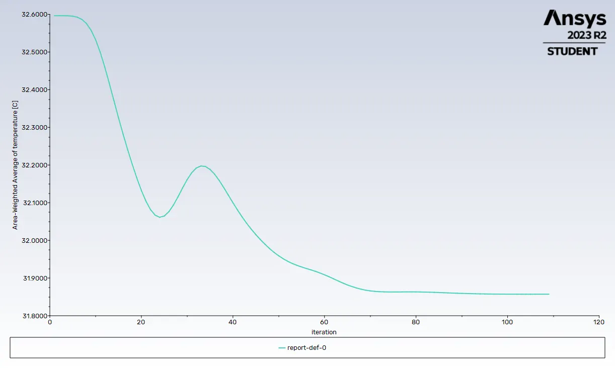
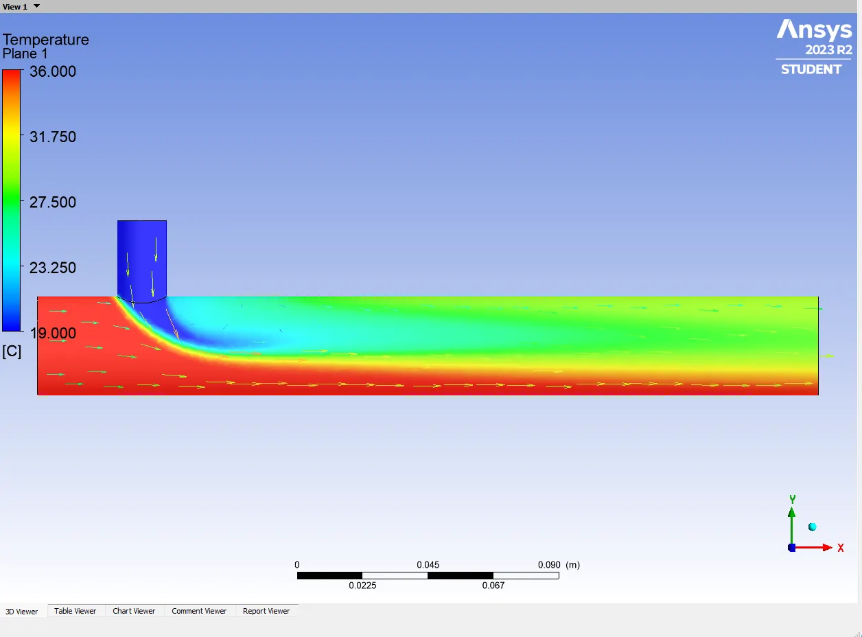
We can see, little more effective mixing at the outlet of the long mixing tee. This occurs because of the diffusion over the length of the pipe.

	Case-1	Case-2
Cell Count	12689	765897
Average Outlet Temperature	33.36 degree C	33.44 degree C
Number of Iterations for convergence	181	106