Week 5.1 - Mid term project - Solving the steady and unsteady 2D heat conduction problem
Week 5.1 - Mid term project - Solving the steady and unsteady 2D heat conduction problem
Objective :-
Solve the 2D heat conduction equation by using the point iterative techniques that were taught in the class.We will implement the following methods for solving implicit equations.The Boundary conditions for the problem are as follows;
Top Boundary = 600 K
Bottom Boundary = 900 K
Left Boundary = 400 K
Right Boundary = 800 K
You will implement the following methods for solving implicit equations.
1. Jacobi
2. Gauss-seidel
3. Successive over-relaxation
absolute error criteria is 1e-4
Solution:-
As We know the equtaion of 2D heat tranfer for steady state and unsedy state.We descretize that equation to find out the values in matrix form and then we solve the matrix by using jacobi,gauss,and successive method in Matlab. There are few things need to be consider before going further it is that for steady state we use implicit method to solve but for unstedy state we need to use both implicit and explicit method.
First we solve for stedy state by using following equation:-
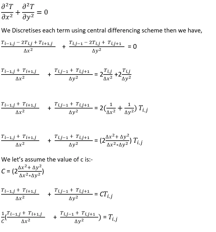
For Jacobi Method,

For Gaussion Method

For Successive over-relaxation

However ω is represent as Relaxation factor which is need to be greter than one for OverRelaxation,and smaller than one for UnderRealxation.
In this case we choose value of ω is 1.2.
Now we begins coding part which was done in matlab to provide sutaible structure of time marchine solution and Itrative methods.
% Steady State 2D Heat Conduction Equation By Jacobi Method
clear all
close all
clc
%Assigning Inputs Values
nx=10;
ny=nx;
x=linspace(0,1,nx);
y=linspace(0,1,ny);
dx=x(2)-x(1);
dy=dx;
%Intial And Boundary Temprtaure
T_b=900;
T_r=400;
T_t=600;
T_l=800;
T(2:nx-1,1)=T_l;
T(2:nx-1,ny)=T_r;
T(nx,2:ny-1)=T_b;
T(1,2:ny-1)=T_t;
%Temparture at corner
T(nx,ny)=(T_b+T_r)/2;
T(nx,1)=(T_l+T_b)/2;
T(1,1)=(T_t+T_l)/2;
T(1,ny)=(T_t+T_r)/2;
%Assigning Value Of T
% T=300*ones(nx,ny);
T_old=T;
%Constant term
c = (dx^2)*(dy^2)/(2*( (dx^2) + (dy^2) ));
%Itrative solver
error=9e9;
tol=1e-4;
%jacobi method
itrative_solver=1;
if itrative_solver==1
tic
jacabo_itr=1;
while (error>tol)
for i=2:nx-1
for j=2:ny-1
T(i,j)=c*((T_old(i-1,j)+T_old(i+1,j))/(dx^2)+(T_old(i,j+1)+T_old(i,j-1))/(dy^2));
end
end
error=max(max(abs(T_old-T)))
T_old=T;
jacabo_itr=jacabo_itr+1;
time_taken=toc
contourf(x,y,T,'ShowText','on')
clabel(contourf(x,y,T))
colorbar
colormap(jet)
set(gca,'ydir','reverse')
xlabel('X-Axis')
ylabel('Y-Axis')
title_txt1=sprintf('number of itration =%d', jacabo_itr)
title_txt2=sprintf('Simulation time =%f', time_taken)
title({'Steady State 2D Heat Conduction Equation By Jacobi Method';title_txt1;title_txt2})
pause(0.03)
end
end
% Steady State 2D Heat Conduction Equation By Gaussion Method
clear all
close all
clc
%Assigning Inputs Values
nx=10;
ny=nx;
x=linspace(0,1,nx);
y=linspace(0,1,ny);
dx=x(2)-x(1);
dy=dx;
%Intial And Boundary Temprtaure
T_b=900;
T_r=400;
T_t=600;
T_l=800;
T(2:nx-1,1)=T_l;
T(2:nx-1,ny)=T_r;
T(nx,2:ny-1)=T_b;
T(1,2:ny-1)=T_t;
%Temparture at corner
T(nx,ny)=(T_b+T_r)/2;
T(nx,1)=(T_l+T_b)/2;
T(1,1)=(T_t+T_l)/2;
T(1,ny)=(T_t+T_r)/2;
%Assigning Value Of T
% T=300*ones(nx,ny);
T_old=T;
%Constant term
c = (dx^2)*(dy^2)/(2*( (dx^2) + (dy^2) ));
%Itrative solver
error=9e9;
tol=1e-4;
%Gaussion method
itrative_solver=1;
if itrative_solver==1
tic
gauss_itr=1;
while (error>tol)
for i=2:nx-1
for j=2:ny-1
T(i,j)=c*((T(i-1,j)+T_old(i+1,j))/(dx^2)+(T(i,j+1)+T_old(i,j-1))/(dy^2));
end
end
error=max(max(abs(T_old-T)))
T_old=T;
gauss_itr=gauss_itr+1;
time_taken=toc
contourf(x,y,T)
clabel(contourf(x,y,T))
colorbar
colormap(jet)
set(gca,'ydir','reverse')
xlabel('X-Axis')
ylabel('Y-Axis')
title_txt1=sprintf('number of itration =%d', gauss_itr)
title_txt2=sprintf('Simulation time =%f', time_taken)
title({'Steady State 2D Heat Conduction Equation By Gaussion Method';title_txt1;title_txt2})
pause(0.03)
end
end
% Steady State 2D Heat Conduction Equation By Successive Over Relaxation method
clear all
close all
clc
%Assigning Inputs Values
nx=10;
ny=nx;
x=linspace(0,1,nx);
y=linspace(0,1,ny);
dx=x(2)-x(1);
dy=dx;
omega=1.2;
%Intial And Boundary Temprtaure
T_b=900;
T_r=400;
T_t=600;
T_l=800;
T(2:nx-1,1)=T_l;
T(2:nx-1,ny)=T_r;
T(nx,2:ny-1)=T_b;
T(1,2:ny-1)=T_t;
%Temparture at corner
T(nx,ny)=(T_b+T_r)/2;
T(nx,1)=(T_l+T_b)/2;
T(1,1)=(T_t+T_l)/2;
T(1,ny)=(T_t+T_r)/2;
%Assigning Value Of T
% T=300*ones(nx,ny);
T_old=T;
%Constant Term
c = (dx^2)*(dy^2)/(2*( (dx^2) + (dy^2) ));
%Itrative solver
error=9e9;
tol=1e-4;
%Successive Over Relaxation method
itrative_solver=1;
if itrative_solver==1
tic
Successive_itr=1;
while (error>tol)
for i=2:nx-1
for j=2:ny-1
term1=(T(i-1,j)+T_old(i+1,j))/dx^2
term2=(T(i,j+1)+T_old(i,j-1))/dy^2
T(i,j)=T_old(i,j)*(1-omega)+omega*c*(term1+term2)
end
end
error=max(max(abs(T_old-T)))
T_old=T;
Successive_itr=Successive_itr+1;
time_taken=toc
contourf(x,y,T)
clabel(contourf(x,y,T))
colorbar
colormap(jet)
set(gca,'ydir','reverse')
xlabel('X-Axis')
ylabel('Y-Axis')
title_txt1=sprintf('number of itration =%d', Successive_itr)
title_txt2=sprintf('Simulation time =%f', time_taken)
title({'Steady State 2D Heat Conduction Equation By Successive Over Relaxation method';title_txt1;title_txt2})
pause(0.03)
end
Outputs:-
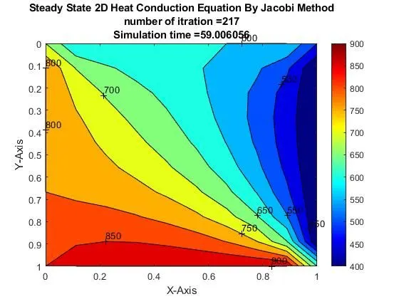
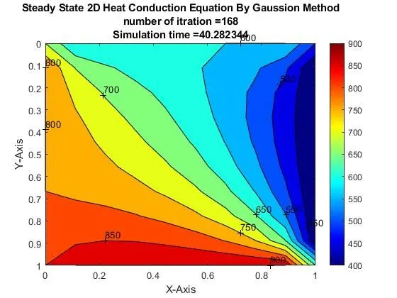
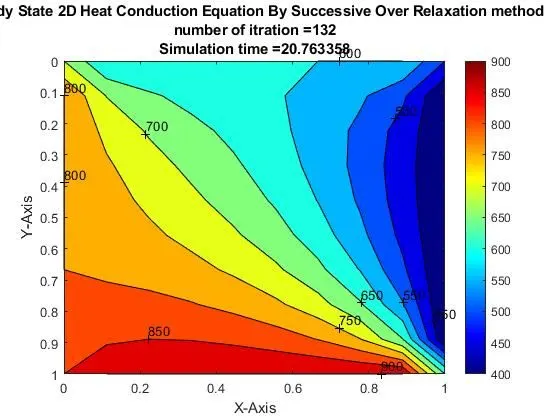
From above results we can clearly see that SOR method is gives less number of iteration than other methods.This method is provide the result in less computational time.
Now we solve for unsteady 2D heat conduction using Implicit iterative:-
As we know the unstedy or transient heat transfer is mens that the temprature is varies with the time.As the time increses the temprature will continue to transfer from one state to another state that's why it's called unstedy state.
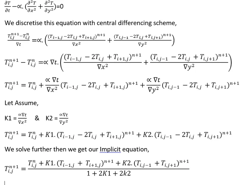
We use following equation and solve it to find out equation for implict and then the matlab use that equation to solve by using jacobian,gaussian and successive over relaxation method.
. 
For Jacobi Method,

For Gaussion Method,

For Successive over-relaxation

However ω is represent as Relaxation factor which is need to be greter than one for OverRelaxation,and smaller than one for UnderRealxation.
In this case we choose value of ω is 1.2.
Now we begins coding part which was done in matlab to provide sutaible structure of time marchine solution and Itrative methods.
% Unsteady State 2D Heat Conduction Equation By Jacobi Method
% Implicit Method
% Jacobi Method
clear all
close all
clc
%Assigning Inputs Values
nx=10;
ny=nx;
nt=300;
x=linspace(0,1,nx);
y=linspace(0,1,ny);
dx=x(2)-x(1);
dy=dx;
dt=0.01; %Number of Time steps
alpha=0.3;
%Intial And Boundary Temprtaure
T_b=900;
T_r=400;
T_t=600;
T_l=800;
T(2:nx-1,1)=T_l;
T(2:nx-1,ny)=T_r;
T(nx,2:ny-1)=T_b;
T(1,2:ny-1)=T_t;
%Temparture at corner
T(nx,ny)=(T_b+T_r)/2;
T(nx,1)=(T_l+T_b)/2;
T(1,1)=(T_t+T_l)/2;
T(1,ny)=(T_t+T_r)/2;
%Assigning Value Of T
% T=300*ones(nx,ny);
T_old=T;
T_prev_dt=T_old;
%Constant term
K1 = ((alpha*dt)/dx^2);
K2 = ((alpha*dt)/dy^2);
%Itrative solver
error=9e9;
tol=1e-4;
%jacobi method
itrative_solver=1;
if itrative_solver==1
tic
jacabo_itr=1;
for k=1:nt %Time loop
error=9e9
while (error>tol)
for i=2:nx-1
for j=2:ny-1
term1=(1+2*K1+2*K2)^-1
term2=term1*K1
term3=term1*K2
h=(T_old(i-1,j)+T_old(i+1,j))
v=(T_old(i,j-1)+T_old(i,j+1))
T(i,j)=(T_prev_dt(i,j)*term1+(term2*h)+(term3*v))
end
end
error=max(max(abs(T_old-T)))
T_old=T
jacabo_itr=jacabo_itr+1;
end
T_prev_dt=T
end
time_taken=toc
figure(1)
contourf(x,y,T,'ShowText','on')
clabel(contourf(x,y,T))
colorbar
colormap(jet)
set(gca,'ydir','reverse')
xlabel('X-Axis')
ylabel('Y-Axis')
title_txt1=sprintf('number of itration =%d', jacabo_itr)
title_txt2=sprintf('Simulation time =%f', time_taken)
title({'Unsteady State Equation By Jacobi Method (Implicit)';title_txt1;title_txt2})
pause(0.03)
end
% Unsteady State 2D Heat Conduction Equation By Gaussian Method
% Implicit method
% Gaussian Method
clear all
close all
clc
%Assigning Inputs Values
nx=10;
ny=nx;
nt=300;
x=linspace(0,1,nx);
y=linspace(0,1,ny);
dx=x(2)-x(1);
dy=dx;
dt=0.01;
alpha=0.3;
%Intial And Boundary Temprtaure
T_b=900;
T_r=400;
T_t=600;
T_l=800;
T(2:nx-1,1)=T_l;
T(2:nx-1,ny)=T_r;
T(nx,2:ny-1)=T_b;
T(1,2:ny-1)=T_t;
%Temparture at corner
T(nx,ny)=(T_b+T_r)/2;
T(nx,1)=(T_l+T_b)/2;
T(1,1)=(T_t+T_l)/2;
T(1,ny)=(T_t+T_r)/2;
%Assigning Value Of T
% T=300*ones(nx,ny);
T_old=T;
T_prev_dt=T_old;
%Constant term
K1 = ((alpha*dt)/dx^2);
K2 = ((alpha*dt)/dy^2);
%Itrative solver
error=9e9;
tol=1e-4;
%Guassian method
itrative_solver=1;
if itrative_solver==1
tic
guass_itr=1;
for k=1:nt
error=9e9
while (error>tol)
for i=2:nx-1
for j=2:ny-1
term1=(1+2*K1+2*K2)^-1
term2=term1*K1
term3=term1*K2
h=(T(i-1,j)+T_old(i+1,j))
v=(T(i,j-1)+T_old(i,j+1))
T(i,j)=(T_prev_dt(i,j)*term1+(term2*h)+(term3*v))
end
end
error=max(max(abs(T_old-T)))
T_old=T
guass_itr=guass_itr+1;
end
T_prev_dt=T
end
time_taken=toc
figure(1)
contourf(x,y,T,'ShowText','on')
clabel(contourf(x,y,T))
colorbar
colormap(jet)
set(gca,'ydir','reverse')
xlabel('X-Axis')
ylabel('Y-Axis')
title_txt1=sprintf('number of itration =%d', guass_itr)
title_txt2=sprintf('Simulation time =%f', time_taken)
title({'Unsteady State Equation By Gaussian Method(Implicit)';title_txt1;title_txt2})
pause(0.03)
end
% Unsteady State 2D Heat Conduction Equation By Successive Over Relaxation method
% Implicit Method
% Successive Over Relaxation method
clear all
close all
clc
%Assigning Inputs Values
nx=10;
ny=nx;
nt=300;
x=linspace(0,1,nx);
y=linspace(0,1,ny);
dx=x(2)-x(1);
dy=dx;
dt=0.01;
alpha=0.3;
omega=1.2;
%Intial And Boundary Temprtaure
T_b=900;
T_r=400;
T_t=600;
T_l=800;
T(2:nx-1,1)=T_l;
T(2:nx-1,ny)=T_r;
T(nx,2:ny-1)=T_b;
T(1,2:ny-1)=T_t;
%Temparture at corner
T(nx,ny)=(T_b+T_r)/2;
T(nx,1)=(T_l+T_b)/2;
T(1,1)=(T_t+T_l)/2;
T(1,ny)=(T_t+T_r)/2;
%Assigning Value Of T
% T=300*ones(nx,ny);
T_old=T;
T_prev_dt=T_old;
%Constant term
K1 = ((alpha*dt)/dx^2);
K2 = ((alpha*dt)/dy^2);
%Itrative solver
error=9e9;
tol=1e-4;
%jacobi method
itrative_solver=1;
if itrative_solver==1
tic
Success_itr=1;
for k=1:nt
error=9e9
while (error>tol)
for i=2:nx-1
for j=2:ny-1
term1=(1+2*K1+2*K2)^-1
term2=term1*K1
term3=term1*K2
h=(T(i-1,j)+T_old(i+1,j))
v=(T(i,j-1)+T_old(i,j+1))
T(i,j)=(T_old(i,j)*(1-omega))+(omega*(T_prev_dt(i,j)*term1+(term2*h)+(term3*v)))
end
end
error=max(max(abs(T_old-T)))
T_old=T
Success_itr= Success_itr+1;
end
T_prev_dt=T
end
time_taken=toc
figure(1)
contourf(x,y,T,'ShowText','on')
clabel(contourf(x,y,T))
colorbar
colormap(jet)
set(gca,'ydir','reverse')
xlabel('X-Axis')
ylabel('Y-Axis')
title_txt1=sprintf('number of itration =%d', Success_itr)
title_txt2=sprintf('Simulation time =%f', time_taken)
title({'Unsteady State Successive Over Relaxation method(Implicit)';title_txt1;title_txt2})
pause(0.03)
end
Outputs:-
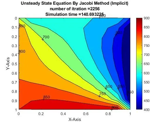
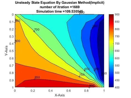
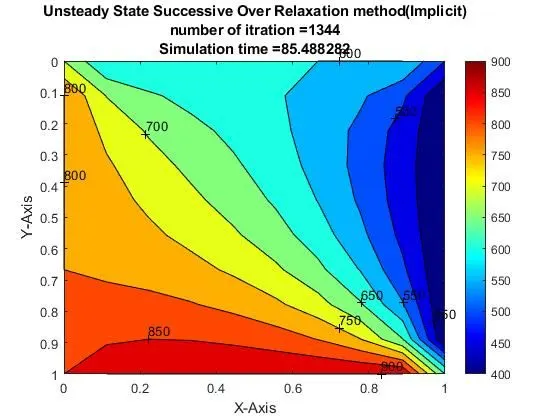
The conclusion of above result is same as the steady state result,the SOR method gives less number of iteration and simulation time than any other method.
unsteady 2D heat conduction using Explicit Method:-
After descretizing we find the equation for explicit schemes,
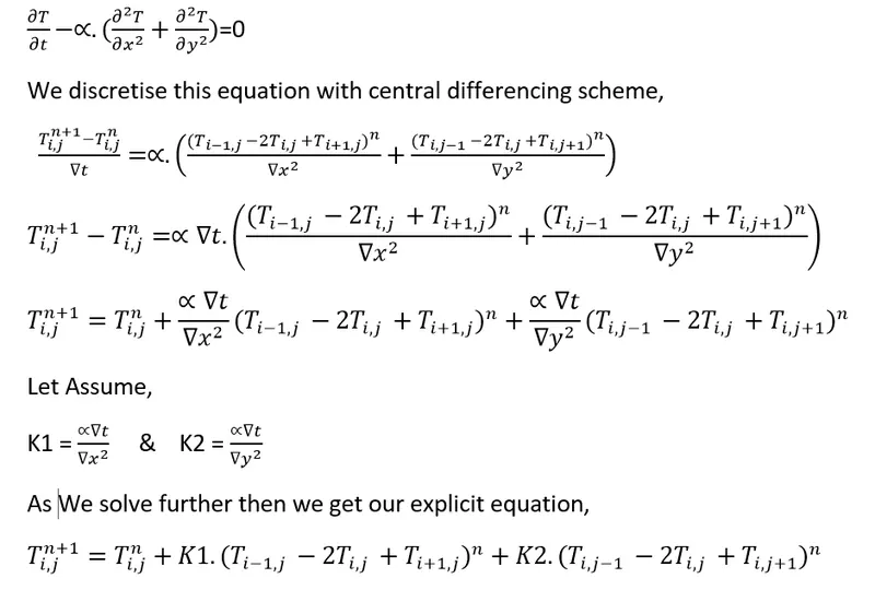
Now we begins coding part which was done in matlab to provide sutaible structure of time marchine solution with Explicit Mathod
% Unsteady State 2D HEat Conduction Equation By Explicit Method
clear all
close all
clc
%Assigning Inputs Values
nx=10;
ny=nx;
nt=300;
x=linspace(0,1,nx);
y=linspace(0,1,ny);
dx=x(2)-x(1);
dy=dx;
dt=0.01;
alpha=0.3;
%Intial And Boundary Temprtaure
T_b=900;
T_r=400;
T_t=600;
T_l=800;
T(2:nx-1,1)=T_l;
T(2:nx-1,ny)=T_r;
T(nx,2:ny-1)=T_b;
T(1,2:ny-1)=T_t;
%Temparture at corner
T(nx,ny)=(T_b+T_r)/2;
T(nx,1)=(T_l+T_b)/2;
T(1,1)=(T_t+T_l)/2;
T(1,ny)=(T_t+T_r)/2;
%Assigning Value Of T
% T=300*ones(nx,ny);
T_old=T;
%T_prev_dt=T_old;
%Constant term
K1 = ((alpha*dt)/dx^2);
K2 = ((alpha*dt)/dy^2);
%Explicit method
tic
Explicit_itr=1;
for k=1:nt
for i=2:nx-1
for j=2:ny-1
term1=(T_old(i-1,j)-2*T_old(i,j)+T_old(i+1,j))
term2=(T_old(i,j-1)-2*T_old(i,j)+T_old(i,j+1))
T(i,j)=T_old(i,j)+K1*(term1)+K2*(term2)
end
end
error=max(max(abs(T_old-T)))
T_old=T
Explicit_it=Explicit_itr+1;
end
time_taken=toc
figure(1)
contourf(x,y,T,'ShowText','on')
clabel(contourf(x,y,T))
colorbar
colormap(jet)
set(gca,'ydir','reverse')
xlabel('X-Axis')
ylabel('Y-Axis')
title_txt1=sprintf('Time =%d', dt*nt)
title_txt2=sprintf('Simulation time =%f', time_taken)
title({'Unsteady State Equation By Explicit Method';title_txt1;title_txt2})
pause(0.03)
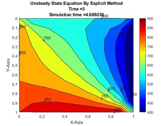
From the above simulation we can see explicit method converge faster than inmplicit method.For steady state we can say SOR mrthod is consider as this method gives faster reslut than any other method.
Explicit method provides less computational period and gives better accuracy.