Week 9 - FVM Literature Review

Week 9 - FVM Literature Review

Finite Volume Method

1. In the finite volume method, instead of writing equation in single point, we are writing the equation in entire volume.
2. In this method we does not assume the shape of a volume, instate we consider the flow that conserved inside the volume this is called the finite volume representation.
3. We write the governing equations in its integral form and then applied gauss divergent theorem, we get discretize form which we are going to solve with using computer.
4. For Finite difference method, we cannot use this method when grind is not alien with x,y and z direction.
5. The advantage of the finite volume method is that it’s easily formulate to allow unstructured mesh and this method is used in many computational fluid dynamics.

Difference between FDM &FVM:

1. A finite volume method discretization is done based on the differential form of PDE to be solve. Each derivative is replaced with an approximate difference formula that can generally be derived from a Taylor series expansion.
2. A finite volume method (FVM) discrecitation is based upon an integral form of PDE to be solved. The PDE is written in a form that can be solved for a given finite volume for cells. The computational domain is discretized into finite volumes and then for every volume, the governing equations are solved. The resulting system of the equation usually involves fluxes of the conserved variables, and thus the calculation of fluxes is very important in FVM
3. The basic advantage of this method over FDM is it does not require the use of structured grids, and the effort to convert the given mesh into a structured numerical grid internally is completely avoided

Interpolation schemes in Finite Volume Method:

Interpolation is a process to estimate the values at unknown points by using the points with known value and sample points on either sides of the unknown point. In FVM, interpolation schemes are used to find values of volume integrals required at the points other than nodes.

Steps:-

1. Once we have this integral form of equation.
2. Apply Gauss divergence theorem
3. We get discretized from which can be solved using computer(‘Flux Terms’)

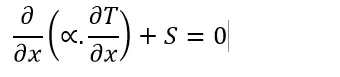
Consider steady state heat equation with heat generation:

Where,

S is source term

`∝` Is thermal diffusivity term

`∂T/∂x`Is temperature gradient along the x direction.

Governing equation 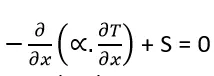is valid at every point in domain. Which means it is also valid in entire control volume.

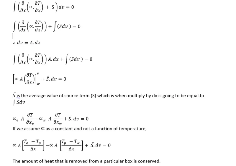
If small control volume (dv) is consider and it is multiplied with the governing equations and integrated if for entire volume then that should be also equal to zero.

Multiplying the equation by ‘dv’ and integrating it –

Different schemas used to solve the equations.

1. Gradient Scheme
2. Interpolation Scheme

1.Gradient Scheme

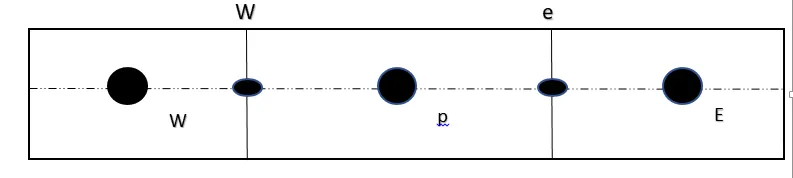
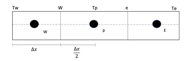
From the above figure when we calculate temperature gradient in the east face, we basically use temperature from neighboring point trying to evaluate or numerically represent gradient of temperature is called as Gradient scheme.

2.Interpolation scheme

In the finite volume formulation, evaluation of surface and volume integrals sometimes requires the values of unknown variables at locations other than the computational nodes of the control volume. These values are obtained by employing certain interpolation schemes. As an example let us consider the simple case of steady one-dimensional convection and diffusion. Where our solution variable (a scalar), p is the density, u is the velocity and r is the diffusion coefficient

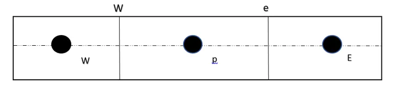
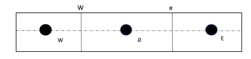
The above figure shows the three neighboring control volumes, which we are going to use for deriving the discretization equation. Integration of the governing differential equation over the control volume around grid point P yields Evaluation of left hand side of the above equation requires the values of 4, over faces e and w. These values are estimated by employing certain interpolation schemes.

Some interpolation schemes used in CFD are as follows:

1. Upwind interpolation scheme
2. Linear interpolation scheme
3. Quadratic Upwind Interpolation for Convective Kinematics (QUICK) scheme
4. Hybrid Scheme
5. Total Variation Diminishing (TVD) scheme

Explaining the Upwind interpolation scheme for an example

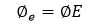
The Upwind interpolation scheme takes into account the direction of fluid flow and based on it, the value of solution variable at the face is approximated by its value at the upstream computational node. For instance, if the fluid is moving from west to east (refer figure), then:

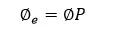
And if the fluid is moving from east to west (refer figure), then:

In addition to these Gradient scheme and interpolation scheme there are flux limiters.

Flux Limiters

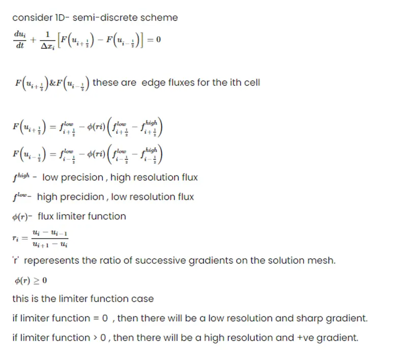
While calculating the variable gradients they tend to toggle and are not bounded to a particular value and keeps jumping, this occurs due to discontinuity due to shock occurring, having a flux limiter will help to bound the gradient value there by giving a stable solution.

Numerical approximation using higher order spatial discretization schemes results in better accuracy but exhibits spurious oscillations near discontinuities such as shocks. On the other hand, lower order spatial discretization schemes remain stable near discontinuities but dampen out the distributionsbecause of their dissipative nature. Hence in order to capture discontinuities, high resolution schemes are desired – which are highly accurate and stable throughout the domain.

Flux limiters operate functionally as a switch and tune the numerical fluxes obtained from lower order scheme and higher order scheme such that near the discontinuity lower order (stable) scheme is employed and away from it higher order (accurate) scheme is employed.

Suppose represents flux at face e calculated using high resolution scheme, L represents flux at e calculated using lower order scheme and H. represents flux at e calculated using higher order scheme. Then b(r) represents the flux limiter function such that:

Flux limiter function depends upon the smoothness parameter r which is defined as

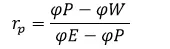
The flux limiter function is constrained to be greater than or equal to zero. It assumes a value of O near discontinuities and a value of 1 away from them. Hence it switches between higher order scheme and lower order scheme for numerical representation of flux, thereby keeping the scheme stable and accurate throughout.

Note that flux limiters are also referred to as slope limiters because they both have the same mathematical form, and both have the effect of limiting the solution gradient near shocks or discontinuities. In general, the term flux limiter is used when the limiter acts on system fluxes and slope limiter is used when the limiter acts on system states (like pressure, velocity etc.).