Week 3.5 - Deriving 4th order approximation of a 2nd order derivative using Taylor Table method

Taylor series

The Taylor series of a function is an infinite sum of terms that are expressed in terms of the functions derivation at a single point. For most common function, the functions and sum of its Taylor series are equal near this point.

As the degree of the Taylor polynomial rises, it approaches the correct function,

Deriving the 4^th order approximation of the second order derivative.

Let’s consider a numerical stenciled with set of grid point as shown in fig.

For right side difference

For Left side difference

For Central side difference

• Skewed 2^nd order right-sided difference scheme

The number of nodes required for 4^th order approximation of a second order derivative can be given by following equation

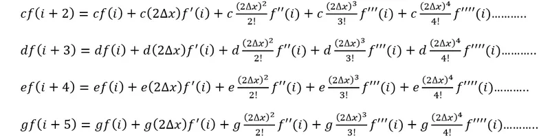
Now, using the Taylor series to find the values of discrete point with respect to point i.

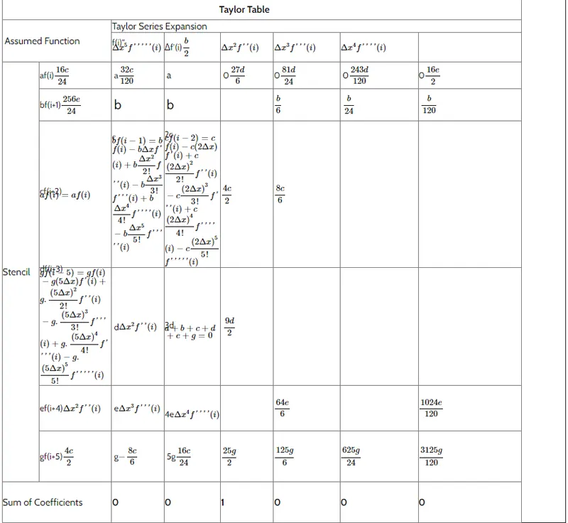
In the above equation, we want only the coefficient of and we assume the coeeficient to be one side and for remaining term we assume the coefficients to be zero.

a + b + c + d + e + g = 0

b + 2c + 3d + 4e + 5g = 0

b/2 + 4c/2 + 9d/2 + 16e/2 + 12g/2 = 0

b/6 + 8c/6 + 27d/6 + 64e/6 + 25g/6 = 0

b/24 + 16c/24 + 81d/24 + 256e/24 + 625g/24 = 0

b/120 + 32c/120 + 243d/120 + 1024e/120 + 3125g/120 = 0

• Skewed 2^nd order Left-sided difference scheme

The number of nodes required for 4^th order approximation of a second order derivative can be given by following equation

Now, using the Taylor series to find the values of discrete point with respect to point i.

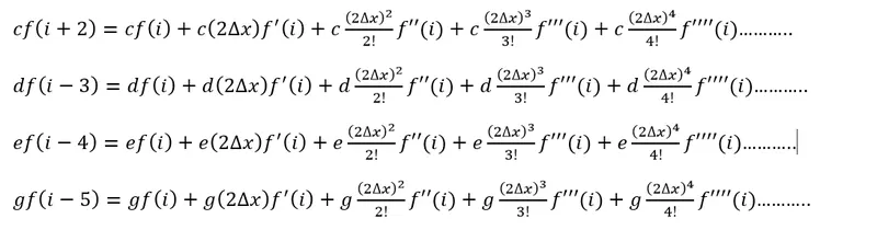
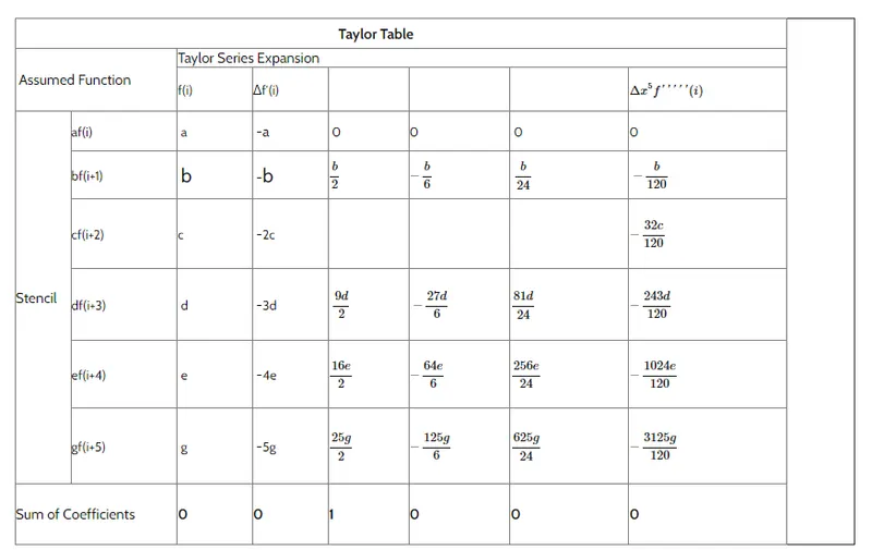
In the above equation, we want only the coefficient of and we assume the coeeficient to be one side and for remaining term we assume the coefficients to be zero.

-(b + 2c + 3d + 4e + 5g) = 0

b/2 + 4c/2 + 9d/2 + 16e/2 + 12g/2 = 1

-(b/6 + 8c/6 + 27d/6 + 64e/6 + 25g/6) = 0

b/24 + 16c/24 + 81d/24 + 256e/24 + 625g/24 = 0

-(b/120 + 32c/120 + 243d/120 + 1024e/120 + 3125g/120) = 0

• Skewed 2^nd order Central difference scheme

The number of nodes required for 4^th order approximation of a second order derivative can be given by following equation

Now, using the Taylor series to find the values of discrete point with respect to point i.

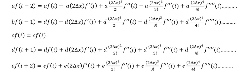
In the above equation, we want only the coefficient of and we assume the coeeficient to be one side and for remaining term we assume the coefficients to be zero.

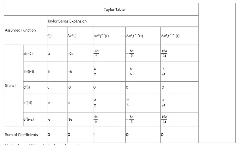
Programing

% second-order derivative of the analytical function exp(x)*cos(x) and compare it with the 3 numerical approximations

clear all
close all
clc
%inputs
x=pi/3;

%stepsize range
dx=linspace(pi/4,pi/400,2000)

%Analytical derivative
%f(x)=exp(x)*cos(x)
%f'(x)=(exp(x)*cos(x)*sin(x)=exp(x)*(cosx-sinx)
%double derivative f"=-2*exp(x)*sin(x);

analytical_derivative = -2*exp(x)*sin(x);
%Right differencing
A=[1 1 1 1 1 1;0 1 2 3 4 5;0 1/2 4/2 9/2 16/2 25/2;0 1/6 8/6 27/6 64/6 125/6;0 1/24 16/24 81/24 256/24 625/24;0 1/120 32/120 243/120 1024/120 3125/120 ]
B=[0;0;1;0;0;0]
x_r=inv(A)*B;
%Left differencing
C=[1 1 1 1 1 1;0 -1 -2 -3 -4 -5;0 1/2 4/2 9/2 16/2 25/2;0 -1/6 -8/6 -27/6 -64/6 -125/6;0 1/24 16/24 81/24 256/24 625/24;0 -1/120 -32/120 -243/120 -1024/120 -3125/120 ]
D=[0;0;1;0;0;0]
x_l=inv(C)*D;
%Centeral differencing
E=[1,1,1,1,1;-2,-1,0,1,2 ;4/2,1/2,0,1/2,4/2;-8/6,-1/6,0,1/6,8/6;16/24,1/24,0,1/24,16/24]
F=[0;0;1;0;0]
x_c=inv(E)*F;

%Anonoymous Function
f=@(x)exp(x).*cos(x);

%Numerical derivation
right_difference =(x_r(1)*f(x)+x_r(2)*f(x+dx)+x_r(3)*f(x+2.*dx)+x_r(4)*f(x+3.*dx)+x_r(5)*f(x+4.*dx)+x_r(6)*f(x+5.*dx))./(dx.^2);
left_difference =(x_l(1)*f(x)+x_l(2)*f(x-dx)+x_l(3)*f(x-2.*dx)+x_l(4)*f(x-3.*dx)+x_l(5)*f(x-4.*dx)+x_l(6)*f(x-5.*dx))./(dx.^2);
cenrer_difference =(x_c(1)*f(x-2.*dx)+x_c(2)*f(x-dx)+x_c(3)*f(x)+x_c(4)*f(x+dx)+x_c(5)*f(x+2.*dx))./(dx.^2);

%Absolute error
error_r=abs(analytical_derivative-right_difference)
error_l=abs(analytical_derivative-left_difference)
error_c=abs(analytical_derivative-cenrer_difference)
error=[error_r;error_l;error_c]

%Plotting
loglog(dx,error_r,"LineWidth",2,"Color",'cyan')
hold on
loglog(dx,error_l,"LineWidth",2,"Color",'b')
hold on
loglog(dx,error_c,"LineWidth",2,"Color",'black')
grid on
ylabel('Abs error')
xlabel('dx')
legend('right difference','left difference','cenrer difference')

Output:-

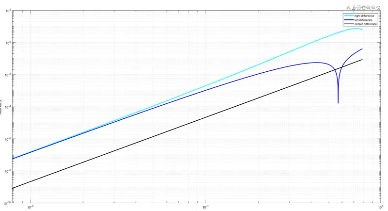
As we can see from the above fig the error for the central difference method is very less compared to the skewed methods.

Skewed right and left difference method almost gives the same result in terms of error for small value of time steps. When data from grid point is only available from either the left or right end i.e. at nodes closer to the boundaries, for computation that requires a high order approximations. we make use of skewed schemes.