Week 7 - Simulation of a 1D Super-sonic nozzle flow simulation using Macormack Method

Simulation of a 1D Super-sonic nozzle flow simulation using Macormack Method

OBJECTIVE:-

1. Steady-state distribution of primitive variables inside the nozzle
2. Time-wise variation of the primitive variables
3. Variation of Mass flow rate distribution inside the nozzle at different time steps during the time-marching process
4. Comparison of Normalized mass flow rate distributions of both forms

1D supersonic nozzle-

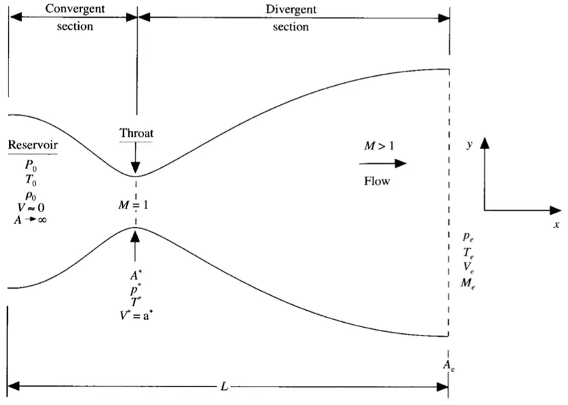
The nozzle has convergent, throat and divergent section. In convergent section when Mach no is less than 1, this condition called subsonic flow. Here the velocity of fluid particle is less than sound speed.

Wherein divergent section when Mach no is greater than 1, this condition is called supersonic flow. Here the velocity of fluid is more than sound speed.

In throat area the Mach no.is equal to 1 that means the speed of sound is equal to fluid particle speed.

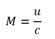
Mach number:-The Mach number is dimensionless quantity representing the ratio of flow velocity past a boundary to the local speed of sound

Where,

M is the Mach number

U is the velocity

C is the speed of sound

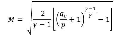
Assuming gas to be an ideal gas, the formula to compute Mach number in a subsonic compressible flow is derived from Bernoulli’s equation.

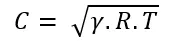
And the speed of sound varies with temperature as

Where,

Is the impact pressure

P is static pressure

Is gamma is the ratio of specific heat to constant pressure

R is the specific gas constant for air

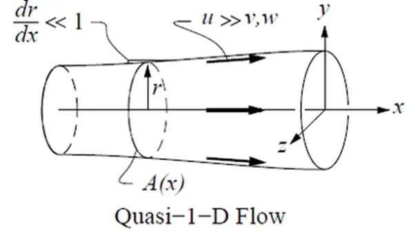
Quasi 1-D Flow

A quasi-One-dimensional flow is one in which all variables vary primarily along with one direction, say x. A flow in duct with slowly-varying area A(x) is the case of interest here.

MacCornac method- The McCormac method is weighted average method which uses both forward differing as well as backward differing schemes to solve the discretized equations.

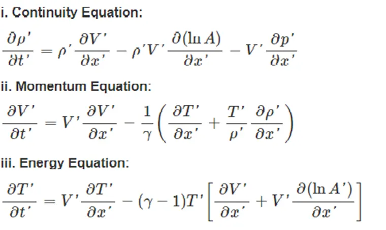
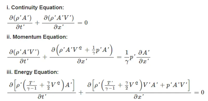
Governing equations:-The supersonic flow through nozzle is governed by novier stroke equations which can be written for both conservative and non-conservative form.

1. Non-conservative form equations

Main program:-

Simulation of a 1D Super-sonic nozzle flow simulation using Macormack Method

%Simulation of a 1D Super-sonic nozzle flow simulation using Macormack Method 
clear all
close all
clc

%Assining input values 
n=31;
x=linspace(0,3,n)
dx=x(2)-x(1);

%Assining area on based on John D. Anderson textbook
A = 1 + 2.2*(x-1.5).^2;
gamma = 1.4
throat = 16
c=0.5;

%Provinding Time steps 
nt=1400;


%soltution by non-conservative form
[rho,T,v,mass_flow_rate_nc,pressure_nc,M,rho_t,T_t,v_t,mass_flow_rate_nc_t,pressure_nc_t,M_t] = non_conservative(x,dx,n,A,nt,gamma,throat)

%solution by consevation form
[rho_c,T_c,v_c,mass_flow_rate_c,p_c,M_c,rho_c_t,T_c_t,v_c_t,mass_flow_rate_c_t,p_c_t,M_c_t] = conservative(x,dx,n,A,gamma,throat)

   %Non-Conservation form
    figure(2)
    title('Steady-state distribution of primitive variables inside the nozzle')
    subplot(4,1,1)
    plot(x,M)
    ylabel('M')
    hold on
    plot(x,M_c,'*')
    legend('Non_conservative','conservative')
    xlabel('x/L')
    grid minor
    
    subplot(4,1,2)
    plot(x,pressure_nc)
    ylabel('p/p')
    hold on
    plot(x,p_c,'*')
     legend('Non_conservative','conservative')
    xlabel('x/L')
    grid minor
    
    subplot(4,1,3)
    plot(x,rho)
    ylabel('rho/rho')
    hold on
    plot(x,rho_c,'*')
     legend('Non_conservative','conservative')
    xlabel('x/L')
    grid minor
    
    subplot(4,1,4)
    plot(x,T)
    ylabel('T/T')
    legend('Non_conservative')
    hold on
    plot(x,T_c,'*')
    legend('Non_conservative','conservative')
    xlabel('x/L')
    grid minor
    
    %Time-wise variation of the primitive variables non-conservation form
    figure(3)
    title('Time-wise variation of the primitive variables non-conservation form')
    subplot(4,1,1)
    plot(1:nt,rho_t)
    ylabel('rho/rho')
    legend('Density')
    axis([0 1400 0 1])
    grid minor
    hold on
    
    subplot(4,1,2)
    plot(1:nt,T_t)
    axis([0 1400 0.6 1])
    ylabel('T/T')
    legend("Temperature")
    grid minor

    
    subplot(4,1,3)
    plot(1:nt,pressure_nc_t)
    ylabel('p/p')
    legend('pressure ratio')
    axis([0 1400 0 1.5])
    grid minor
    
    subplot(4,1,4)
    plot(1:nt,M_t)
    ylabel('M')
    legend('Mach Number')
    axis([0 1400 0.6 2])
    grid minor
    
    %Time-wise variation of the primitive variables conservative form
    figure(4)
    title('Time-wise variation of the primitive variables conservative form')
    subplot(4,1,1)
    plot(1:nt,rho_c_t,'r')
    ylabel('rho/rho')
    legend('Density')
    axis([0 1400 0 1])
    grid minor
    hold on
    
    subplot(4,1,2)
    plot(1:nt,T_c_t,'r')
    axis([0 1400 0.6 1])
    ylabel('T/T')
    legend("Temperature")
    grid minor
    hold on
    
    subplot(4,1,3)
    plot(1:nt,p_c_t,'R')
    ylabel('p/p')
    legend('pressure ratio')
    axis([0 1400 0 1.5])
    grid minor
    
    subplot(4,1,4)
    plot(1:nt,M_c_t,'r')
    ylabel('M')
    legend('Mach Number')
    axis([0 1400 0.6 2])
    grid minor

    
 %plot for conservation vs non conservattion form
 figure (7)
 plot(x,mass_flow_rate_nc)
 hold on
 plot(x,mass_flow_rate_c,'Color','R')
 xlabel('x/L')
 ylabel('rhoVA/rho_{o}v_{o}A_{o}')
 title('mass flow rate comparison between the conservation form and non-conservation form')
 grid on
 grid minor

After obtaining the Non-conservative form of governing equations, the following steps nedds to consider:-

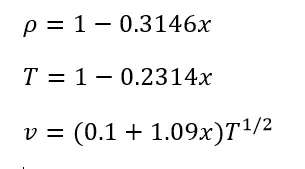
Step 1: Initial condition

The nozzle shape, A =A(x),is specified and held fixed, independent of time.

For density, Temperature and velocity is given by

Step 2: Predictor steps

In continuity equation, replace the spatial derivative on right hand side with forward difference

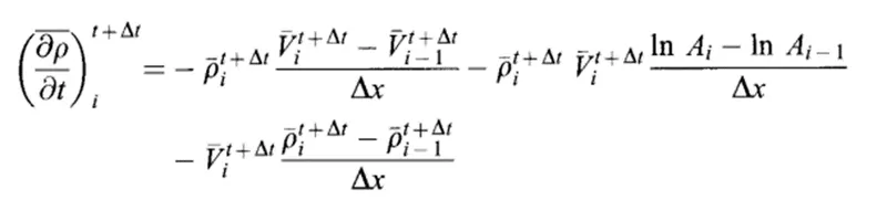
In above equation, all flow variables at time t are known.

Predicted value from the first two terms of a taylor series

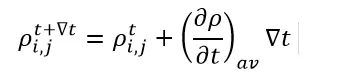
Similar equations can be written for predicted values of other variables

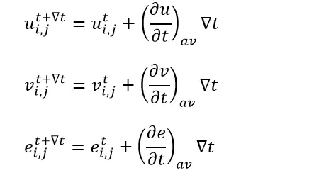
Step 3: Corrector steps

We first obtain the predicted value of the time derivative at time t+ by substituting values the predicator values of rho, u and v into right side of the continuity equation.

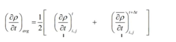
Step 4: Average value

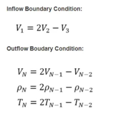
Step 5 : Boundary conditions

Function for Non-conservative form of governing equations

function [rho,T,v,mass_flow_rate_nc,pressure_nc,M,rho_t,T_t,v_t,mass_flow_rate_nc_t,pressure_nc_t,M_t] = non_conservative(x,dx,n,A,nt,gamma,throat)
%Assining intial values of primitive variables
rho = 1-0.3146*x;
T = 1-0.2314*x;
v = (0.1 + 1.09*x).*T.^0.5;
mass_flow_rate_nc = rho.*A.*v; %mass flow rate
pressure_nc = rho.*T;          %pressure 
M = v./sqrt(T); 
c=0.5;           
dt=min((c.*dx./(sqrt(T)+v)));

%Values at throat
rho_t=rho(throat);
v_t = v(throat);
T_t = T(throat);
mass_flow_rate_nc_t=mass_flow_rate_nc(throat);
pressure_nc_t=pressure_nc(throat);
M_t=M(throat);

%Now we begins Time loop
for i=1:nt
    rho_old =rho;
    v_old =v;
    T_old = T;
    % predictor step
    for j=2:n-1
        dv_dx_p = ((v(j+1)-v(j))/dx);
        dlogA_dx_p= ((log(A(j+1))-log(A(j)))/dx);
        drho_dx_p = ((rho(j+1)-rho(j))/dx);
        dT_dx_p = ((T(j+1)-T(j))/dx);
        %continuty Equation
        drho_dt_p(j) = -rho(j)*dv_dx_p-rho(j)*v(j)*dlogA_dx_p- v(j)*drho_dx_p;
        %momentum equation
        dv_dt_p(j) = -v(j)* dv_dx_p-(1/gamma)*(dT_dx_p+(T(j)/rho(j))* drho_dx_p);
        %Energy equation
        dT_dt_p(j) = -v(j)* dT_dx_p-(gamma-1)*T(j)*(dv_dx_p + v(j)* dlogA_dx_p);
        %solution update 
        rho(j)=rho(j) +  drho_dt_p(j)*dt;
        v(j) = v(j)   +  dv_dt_p(j)*dt;
        T(j) = T(j)   +  dT_dt_p(j)*dt;
    end
    %corrector step
    for j=2:n-1
        dv_dx_c = ((v(j)-v(j-1))/dx);
        dlogA_dx_c= ((log(A(j))-log(A(j-1)))/dx);
        drho_dx_c = ((rho(j)-rho(j-1))/dx);
        dT_dx_c = ((T(j)-T(j-1))/dx);
        %continuty Equation
        drho_dt_c(j) = -rho(j)*(dv_dx_c)-rho(j)*v(j)*( dlogA_dx_c)- v(j)* drho_dx_c;
        %momentum equation
        dv_dt_c(j) = -(v(j)* dv_dx_c)-((1/gamma)*( dT_dx_c+(T(j)/rho(j))* drho_dx_c));
        %Energy equation
        dT_dt_c(j) = -(v(j)* dT_dx_c)-((gamma-1)*T(j)*(dv_dx_c + v(j)* dlogA_dx_c));
    end
    % compute the avarage time derivative
    drho_dt_avg = 0.5*( drho_dt_p +  drho_dt_c);
    dv_dt_avg =0.5*( dv_dt_p +   dv_dt_c);
    dT_dt_avg = 0.5*( dT_dt_p +  dT_dt_c);
    
    %final solution update 
    for k=2:n-1
        rho(k)=rho_old(k)+   drho_dt_avg(k)*dt;
        v(k) = v_old(k) +   dv_dt_avg(k)*dt;
        T(k) = T_old(k) +   dT_dt_avg(k)*dt;
    end
    
    %boundary condition
    %inlet
    v(1)=2*v(2)-v(3);
    %outlet
    rho(n)=2*rho(n-1)-rho(n-2);
    v(n)=2*v(n-1)-v(n-2);
    T(n)=2*T(n-1)-T(n-2);
    
    %At throat
    throat = ((n+1)/2);
    
    %Defining mass flow rate
    mass_flow_rate_nc = rho.*A.*v; %mass flow rate
    pressure_nc = rho.*T;          %pressure 
    M = v./sqrt(T);                %mach number
    
    %Values at throat
    rho_t(i)=rho(throat);
    v_t(i) = v(throat);
    T_t(i) = T(throat);
    mass_flow_rate_nc_t(i)=mass_flow_rate_nc(throat);
    pressure_nc_t(i)=pressure_nc(throat);
    M_t(i)=M(throat);
    
    if i==50
        figure(5)
        plot(x,mass_flow_rate_nc)
        hold on
        figure(5)
    elseif i==100
        plot(x,mass_flow_rate_nc)
    elseif i==150
        plot(x,mass_flow_rate_nc)
    elseif i==200
        plot(x,mass_flow_rate_nc)
     elseif i==550
        plot(x,mass_flow_rate_nc) 
     elseif i==700
        plot(x,mass_flow_rate_nc)
     elseif i==1400
        plot(x,mass_flow_rate_nc)
    end
    title(sprintf('Time steps=%d',i))
    xlabel('x/L')
    ylabel('rhoVA/rho_{o}v_{o}A_{o}')
    legend('50Deltat','100Deltat','150Deltat','200Deltat','550Deltat','700Deltat','1400Deltat')
    axis([0 3 0.4 1.6])
    grid on
    grid minor
end

end

Conservative Form

The basic equation in conservative form

The equations for quasi-one-dimensional flow can be expressed in a similar generic form. Let us define the elements of the solution vector U, the flux matrix F, and the source terms J as follows

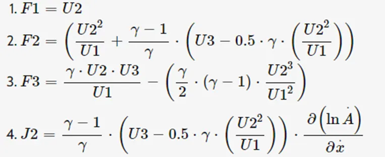
Conversed form complex into simpler form

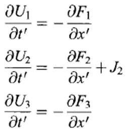
Now we can solve similar to non-conservative approach

Boundary conditions

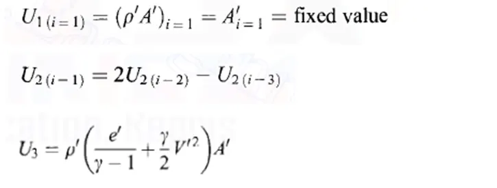
Inlet Boundary conditions

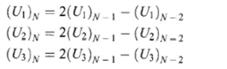
Outlet Boundary conditions

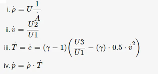
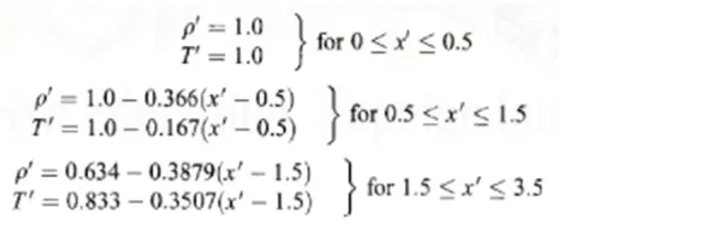
Initial Condition:-The initial condition are provided in terms of primitive variables

Calculating the time step by using same approach as in the non-conservative form.

Function for conservative form of governing equations

function [rho_c,T_c,v_c,mass_flow_rate_c,p_c,M_c,rho_c_t,T_c_t,v_c_t,mass_flow_rate_c_t,p_c_t,M_c_t] = conservative(x,dx,n,A,gamma,throat)
%Initilaization step
%initializing density and temperature
for i=1:length(x)
    if x(i)<=0.5
        
       rho_c(i) = 1.0;
       T_c(i) = 1.0;
       
    else if x(i)>=0.5 && x(i)<= 1.5
           
           rho_c(i) = 1-0.366*(x(i)-0.5);
           T_c(i) = 1-0.167*(x(i)-0.5); 
           
    else if x(i)>=1.5 && x(i)<= 3.0
            
            rho_c(i) = 0.634-0.3879*(x(i)-1.5);
            T_c(i)  = 0.833-0.3507*(x(i)-1.5); 
    end
    end
    end
end
        
%Initializing the solution vector
%velocity
v_c = 0.59./(rho_c.*A);

%pressure
p_c = rho_c.*T_c;

%mass Flow rate
mass_flow_rate_c=rho_c.*A.*v_c;

%Mach Number
M_c = v_c./(T_c.^0.5);

%Values at throat
 rho_c_t=rho_c(throat);
 v_c_t = v_c(throat);
 T_c_t = T_c(throat);
 mass_flow_rate_c_t=mass_flow_rate_c(throat);
 p_c_t=p_c(throat);
 M_c_t=M_c(throat);

% Intialization of solution vector
U1 = rho_c.*A;
U2 = rho_c.*A.*v_c;
U3 = rho_c.*A.*((T_c./(gamma-1))+ (gamma/2).*(v_c.^2));

%Provinding Time steps 
c=0.5;
nt=1400;
dt=min((c.*dx./(sqrt(T_c)+v_c)));

%Time toop
for k=1:nt
   % Preserving the old solution vector 
    U1_old = U1;
    U2_old = U2;
    U3_old = U3;
    
    %Defining the flux vector
    F1 = U2;
    F2 = ((U2.^2)./U1) + ((gamma-1)/gamma).*(U3-(gamma/2).*((U2).^2./U1));
    F3 = ((gamma.*U2.*U3)./U1) - ((gamma*(gamma-1))./2).*((U2.^3)./(U1.^2));
   
    for j=2:n-1
    %Definining the source term
    J2(j)=(1/gamma)*rho_c(j)*T_c(j)*((A(j+1)-A(j))/dx);
    
    % predictor steps
    dU1_dx_p = (F1(j+1)-F1(j))/dx;
    dU2_dx_P = (F2(j+1)-F2(j))/dx;
    dU3_dx_p = (F3(j+1)-F3(j))/dx;
    
    dU1dt_p(j) = -(dU1_dx_p);
    dU2dt_p(j) = -(dU2_dx_P)+ J2(j);
    dU3dt_p(j) = -(dU3_dx_p);
    
    %Updating the new value of solution vector
    U1(j)= U1_old(j) +  dU1dt_p(j)*dt;
    U2(j)= U2_old(j) +  dU2dt_p(j)*dt;
    U3(j)= U3_old(j) +  dU3dt_p(j)*dt;
    
    %Updataion of primiive variables
    rho_c(j)=U1(j)./A(j);
    v_c(j) = U2(j)./U1(j);
    T_c(j) = (gamma-1).*((U3(j)./U1(j))-((gamma./2).*(v_c(j).^2)));
    p_c(j) = rho_c(j).*T_c(j);
    end
   
   %Defining the flux vector
    F1 = U2;
    F2 = ((U2.^2)./U1) + ((gamma-1)./gamma).*(U3-(gamma./2).*((U2).^2./U1));
    F3 = ((gamma.*U2.*U3)./U1) - ((gamma.*(gamma-1))./2).*((U2.^3)./(U1.^2));
    
    %corector step
    for j=2:n-1
        
    %Definining the source term
    J2(j)=(1/gamma)*rho_c(j)*T_c(j)*((A(j)-A(j-1))/dx);
    
    % corector steps
    dU1_dx_c = (F1(j)-F1(j-1))/dx;
    dU2_dx_c = (F2(j)-F2(j-1))/dx;
    dU3_dx_c = (F3(j)-F3(j-1))/dx;
    
    dU1dt_c(j) = -dU1_dx_c;
    dU2dt_c(j) = -dU2_dx_c + J2(j);
    dU3dt_c(j) = -dU3_dx_c;
    end
    
    % compute the avarage time derivative
    dU1dt = 0.5.*(dU1dt_p +  dU1dt_c);
    dU2dt = 0.5.*(dU2dt_p +  dU2dt_c);
    dU3dt = 0.5.*(dU3dt_p +  dU3dt_c);
    
    %final solution update 
    for g=2:n-1
        U1(g) = (U1_old(g) + dU1dt(g)*dt);
        U2(g) = (U2_old(g) + dU2dt(g)*dt);
        U3(g) = (U3_old(g) + dU3dt(g)*dt);
    end
    %boundary condition
    %inlet
    U1(1) = rho_c(1)*A(1);
    U2(1) = 2*U2(2)-U2(3);
    U3(1) = U1(1)*(T_c(1)/(gamma-1)+(0.5*gamma)*v_c(1).^2);
    %outlet
    U1(n)=2*U1(n-1)-U1(n-2);
    U2(n)=2*U2(n-1)-U2(n-2);
    U3(n)=2*U3(n-1)-U3(n-2);
    
    %Updataion of primiive variables
    rho_c=U1./A;
    v_c = U2./U1;
    T_c = (gamma-1)*((U3./U1)-(gamma/2)*v_c.^2);
    
    %calculating pressure,mach number and mass flow rate
    p_c = rho_c.*T_c;
    mass_flow_rate_c = rho_c.*A.*v_c;
    M_c = v_c./(sqrt(T_c));
    
    %Values at throat
    rho_c_t(k)=rho_c(throat);
    v_c_t(k) = v_c(throat);
    T_c_t(k) = T_c(throat);
    mass_flow_rate_c_t(k)=mass_flow_rate_c(throat);
    p_c_t(k)=p_c(throat);
    M_c_t(k)=M_c(throat);
   
    %Mass flow rate across the nozzle at different time steps
    figure(1)
    if k==100
        plot(x,mass_flow_rate_c)
        hold on
    elseif k==150
        plot(x,mass_flow_rate_c)
        hold on
     elseif k==200     
        plot(x,mass_flow_rate_c)
        hold on
     elseif k==550     
        plot(x,mass_flow_rate_c)
        hold on
     elseif k==700     
        plot(x,mass_flow_rate_c)
        hold on
     elseif k==1400     
        plot(x,mass_flow_rate_c)
        hold on
    end
    title(sprintf('Time steps=%d',k))
    xlabel('x/L')
    ylabel('rhoVA/rho_{o}v_{o}A_{o}')
    legend('50Deltat','100Deltat','150Deltat','200Deltat','550Deltat','700Deltat','1400Deltat')
    axis([0 3 0.4 1.6])
    grid on
    grid minor
end
end

Results:-

1 .The variable inside the nozzle is plotted using conservation and non-conservation form and compared them with each other.

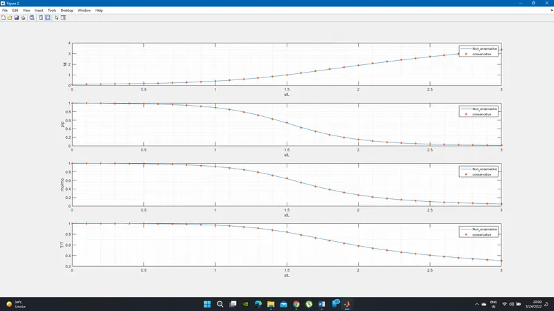
It shows that both forms return to its identical profile for mach number density velocity and Pressure and temperature. The mass flow rate is more unstable in non-conservative form.

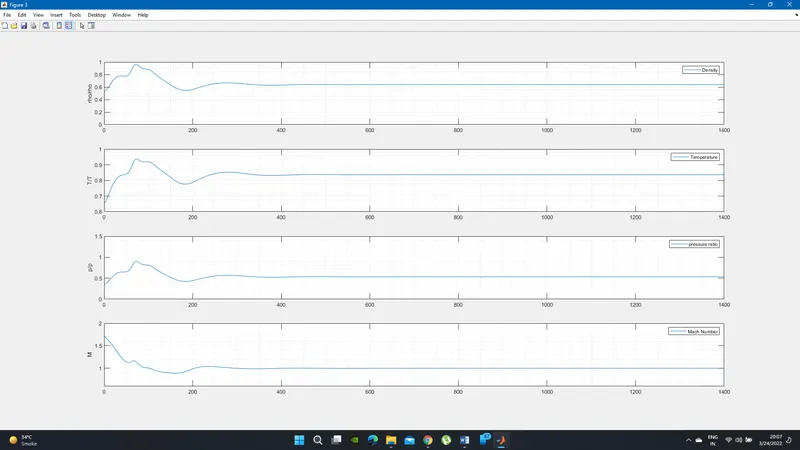
2. Time wise variation of primitive variables using non-conservative equations

3. Time wise variation of primitive variables using conservative equations

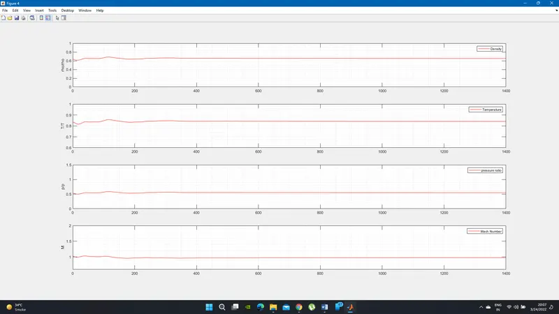
The graph is plotted for density temperature and pressure and Mach number.

Initially the values of the parameters are high and oscillate, this occurs due to various effects on flow such as compression and expansion which occurs in nozzle.

And in upcoming steps the values are approaching near to stability and constant condition.

It can be seen that there are more oscillation occurs in 0-200 time steps and gradually decrease from 200-400 time steps

From the plot we can also see that the minimum number of cycle to run is 600 for convergence.

It can be said that the conservative from has less oscillation then non conservative form.

4. Variation of Mass flow rate distribution inside the nozzle at different time steps during the time-marching process for non-conservative form

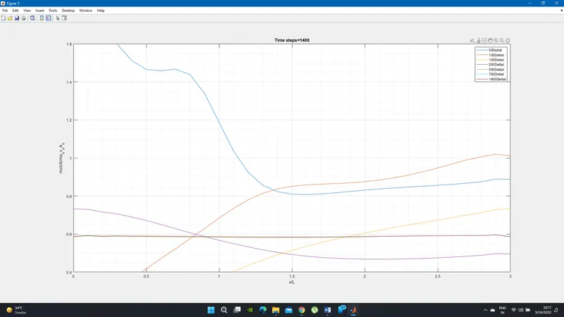
The variation of mass flow rate at different time steps for non-conservation form.7 different time steps are taken and shown in graph which depicts different mass flow rate at different time steps Mass flow rate varies from convergent section to divergent section for the earlier time steps. After achieving a steady state which is in between 500 to 700 steps variation in mass flow rate decreases.

5. Variation of Mass flow rate distribution inside the nozzle at different time steps during the time-marching process for conservative form

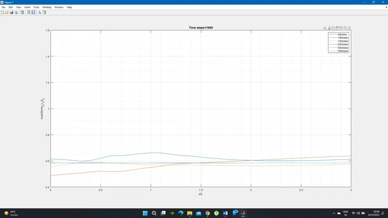
It shows that at initial time marching as the time derivative are quite large the mass flow rate appears to be very high throughout the length of nozzle. But after 200 time steps the value is approaching steady state and at 700 times steps we can say that the value is converged

6. Plot for the mass flow rate comparison between the conservation form and non-conservation form

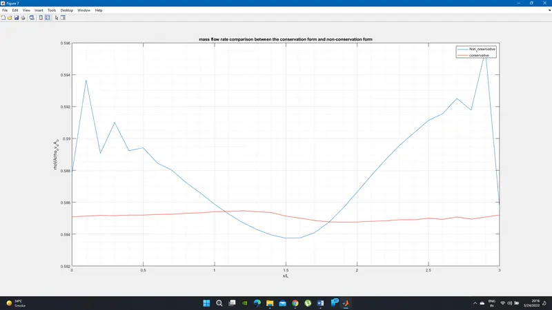
The mass flow rate variation is more in the non-conservative form as compare to the conservative form where mass flow rate more or less constant through the length of the nozzle

Grid Dependence Test:-

Here rho, T, P represent initial values of pressure temperature and density while rho_t, T_t ,P_t represent the value at throat.

The two grid point are consider as n=31 and n=61 while as throat values are taken at i=16

From the table it can be seen that as we increase the number of grid point the values of variables approach towards exact solution but change is marginal. But increase in number of grid point also increase for both form.

From the result we can say that the non-conservation form is much slower than the conservation forms.

Accuracy increases with grid point increases and time for simulation also increases.

Conclusion

1. Simulation time increases with increase in grid point and accuracy also increases.
2. Non conservation form is then faster than conservation form
3. Mass flow distribution is better in conservation form then in non-conservation form.
4. Initially at lower time steps there are oscillation’s in the solution but as the time step increases the solution moves to steady state and converge near to 800 time steps
5. So the solution must be run at least up to 800 time steps for it to converge