Week 1- Mixing Tee

MIXING TEE

AIM: to set up steady-state simulations to compare the mixing effectiveness when the hot inlet temperature is 36⁰C & the Cold inlet is at 19⁰C creating two versions of the mixing tee.

OBJECTIVE:

• is to set up steady-state simulations to compare the mixing effectiveness when the hot inlet temperature is 36⁰C & the Cold inlet is at 19⁰C.
• Use the k-epsilon and k-omega SST model for the first case and based on your judgment use the more suitable model for further cases. Giving the reason for choosing a suitable model is compulsory.

1. Case 1
   • Short mixing tee with a hot inlet velocity of 3m/s.
   • Momentum ratio of 2, 4.
2. Case 2
   • Long mixing tee with a hot inlet velocity of 3m/s.
   • Momentum ratio of 2, 4.

• Momentum ratio = velocity at cold inlet / velocity at hot inlet
• In a table, compare the following values from the 2 cases.

1. Cell count
2. Average outlet temperature
3. Number of iterations for convergence

• Expected results:

1. Velocity and temperature contour plots on the cut planes along and across the pipe.
2. Velocity and temperature line plots along and across the length of the pipe.
3. Perform Mesh independent study for any one case.
4. Discuss the effect of length and momentum ratio on results.

PROCEDURE AND RESULTS:

1. Case 1
   • Short mixing tee with a hot inlet velocity of 3m/s.
   • Momentum ratio of 2, 4

In case 1 we are doing two different sub-cases one being the velocity of cold air 6m/s and another being 12m/s

Subcase 1:

Geometry:

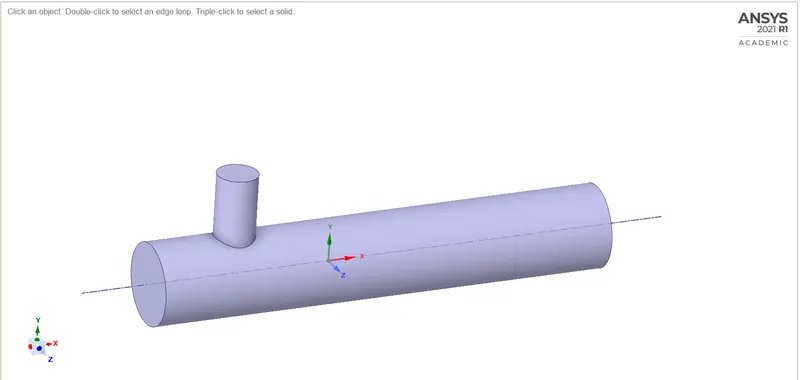
The Geometry has been provided in the challenge interface. The first case is simulated with the short T-joint with the momentum ratio 2.

Meshing:

We have done mesh refinement by an element size = 0.002m and keeping the rest of it default

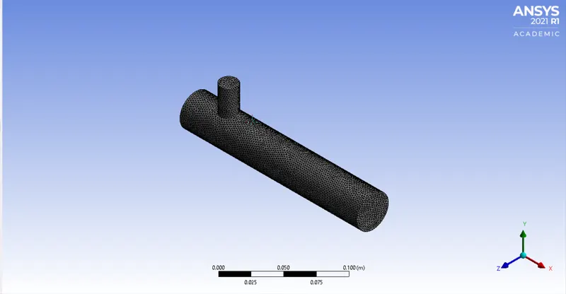
with an element quality of:

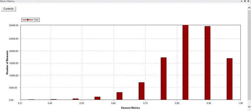
and the number of elements and nodes :

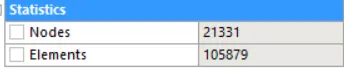
After creating the Mesh file, we name the geometry for the further use

1. Inlet x (inlet where the hot air come from)

2. Inlet y (inlet where the cold air come from)

3. The walls

4. Outlet

After updating the mesh file we go to the solution part.

Solution

SETUP	Short TEE (MR=4 & Inlet Hot Velocity=3m/s)
	K-epsilon	K-omega
Solver Type	Pressure Based	Pressure Based
Velocity Formulation	Absolute	Absolute
Time	Steady	Steady
Viscous Model	Realizable k-epsilon with standard wall function	k-omega SST model
Material	Air	Air
Cell zones Volume_volume	Fluid type: Air	Fluid type: Air
Boundaries	Inlet x (velocity inlet) Velocity Magnitude 3m/s Temperature – 36 degrees c. Inlet y (velocity inlet) Velocity Magnitude 6m/s Temperature – 19 degrees c. Outlet x (Pressure outlet) Gauge Pressure – 0 pas. Walls – Stationary walls	Inlet x (velocity inlet) Velocity Magnitude 3m/s Temperature – 36 degrees c. Inlet y (velocity inlet) Velocity Magnitude 6m/s Temperature – 19 degrees c. Outlet x (Pressure outlet) Gauge Pressure – 0 pas. Walls – Stationary walls

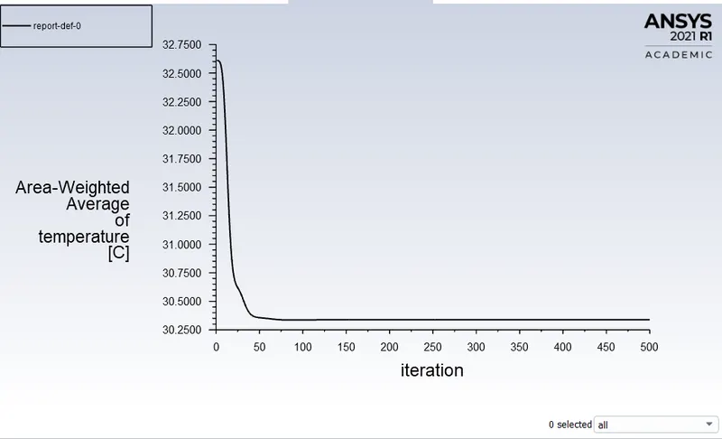
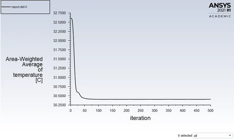
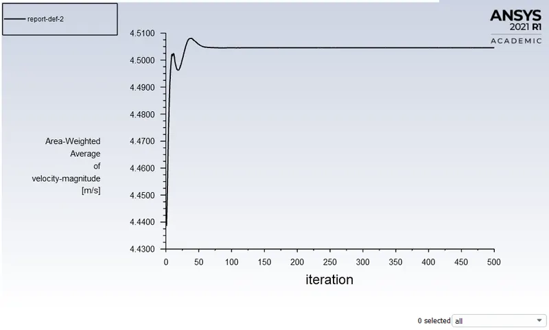
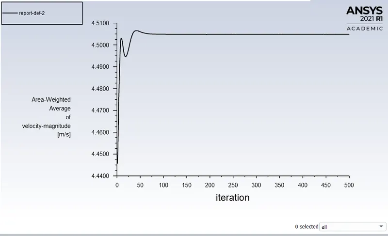
Left being k-epsilon and the right being the k-omega

Residuals Plot

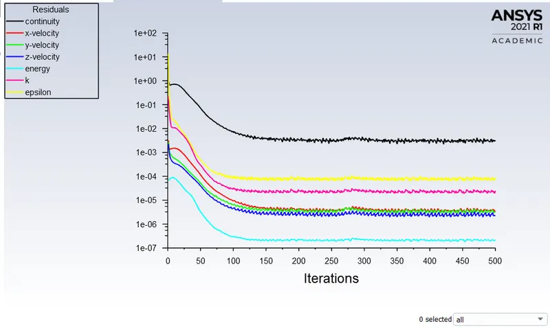
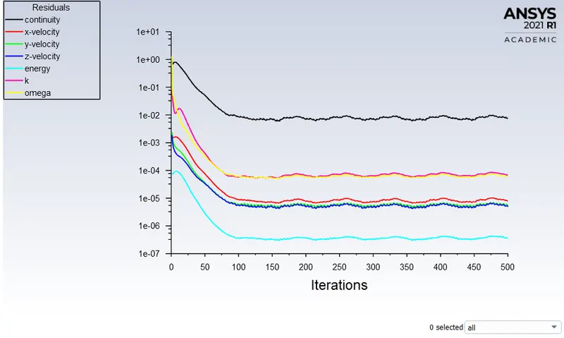
Average weighted area Plot to find the outlet Temperature

Standard Deviation Plot to find the Effectiveness of Mixing at the outlet

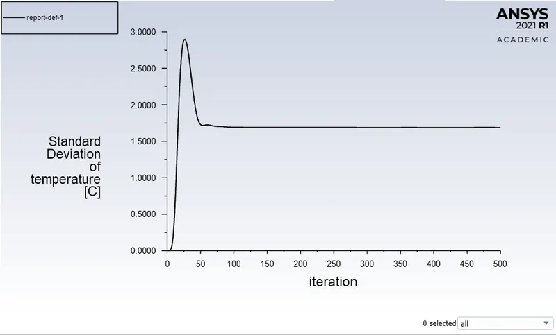
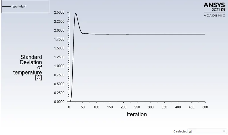
Average weighted area Plot to find the outlet Velocity

Countor Plot

1)For Temperature distribution

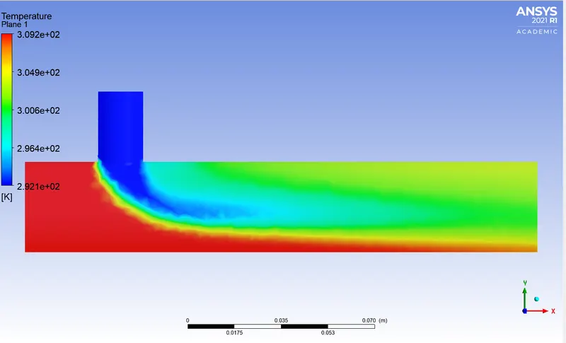
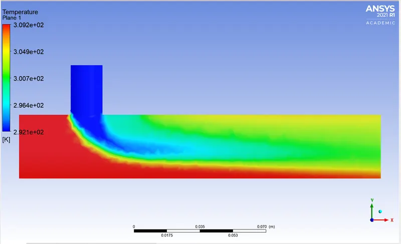
2)For Velocity Distribution

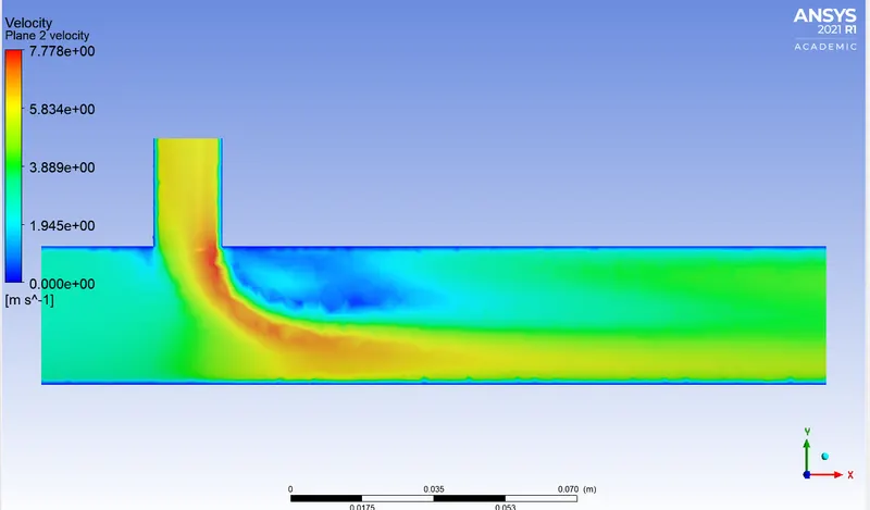
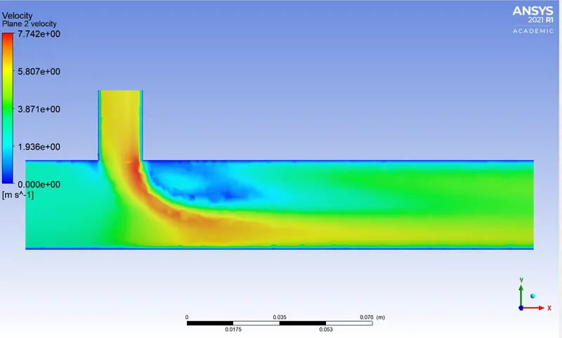
The flow of air in a pipe animation:

https://youtu.be/GU0jN1yzQ24

Subcase 2:

For velocity of hot air 3m/s and cold air 12m/s

In which geometry and the mesh is the same as the previous one. Only the solution part changes i.e, the boundary conditions where the inlet y changes from 6 to 12 m/s

SETUP	K-epsilon
Solver Type	Pressure Based
Velocity Formulation	Absolute
Time	Steady
Viscous Model	Realizable k-epsilon with standard wall function
Material	Fluid type: Air
Cell zones Volume_volume	Fluid type: Air
Boundaries	Inlet x (velocity inlet) Velocity Magnitude 3m/s Temperature – 36 degrees c. Inlet y (velocity inlet) Velocity Magnitude 6m/s Temperature – 19 degrees c. Outlet x (Pressure outlet) Gauge Pressure – 0 pas. Walls – Stationary walls

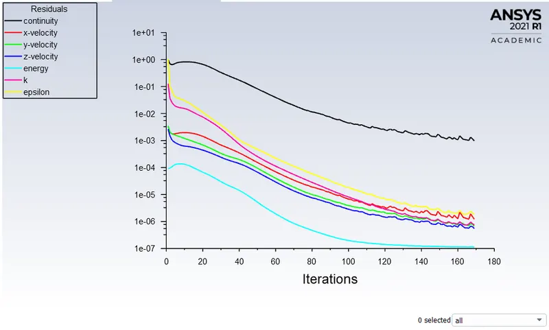
Residuals Plot

Average weighted area Plot to find the outlet Temperature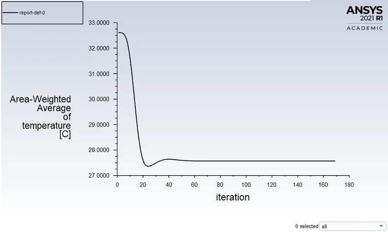

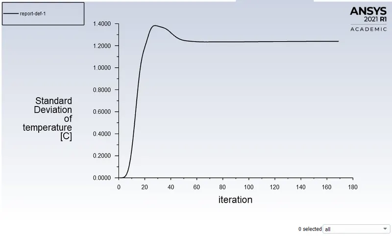
Standard Deviation Plot to find the Effectiveness of Mixing at the outlet

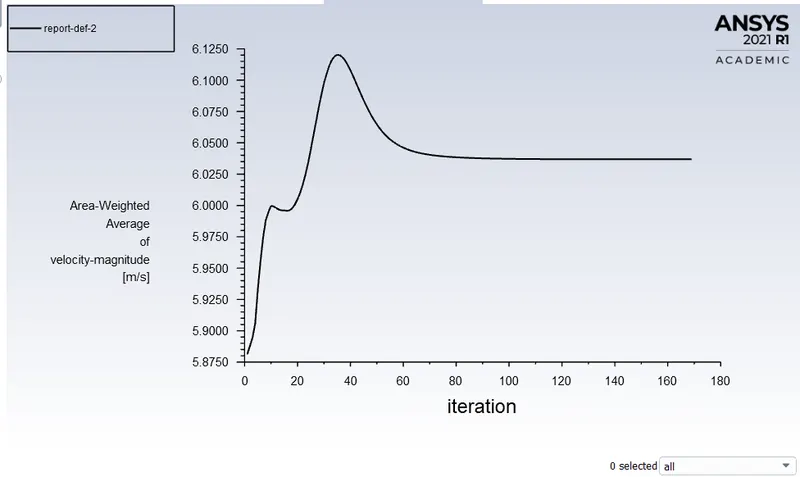
Average weighted area Plot to find the outlet Velocity

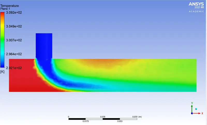
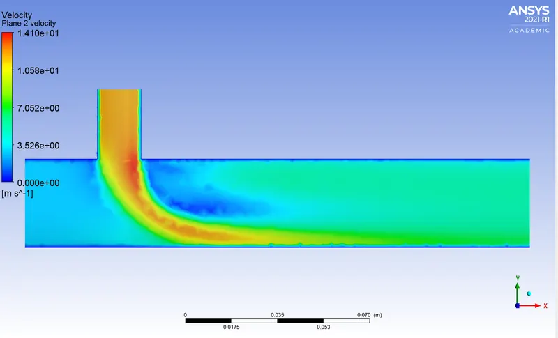
Countor Plot

1)For Temperature distribution

2)For Velocity Distribution

The flow of air in a pipe animation:

https://youtu.be/E9ibHFMRrbs

CASE 2:

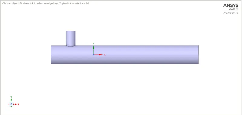
Geometry

The Geometry has been provided in the challenge interface. The first case is simulated with the short T-joint with the momentum ratio 2.

Meshing:

We have done mesh refinement by an element size = 0.002m and keeping the rest of it default

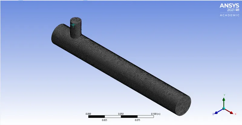
with an element quality of:

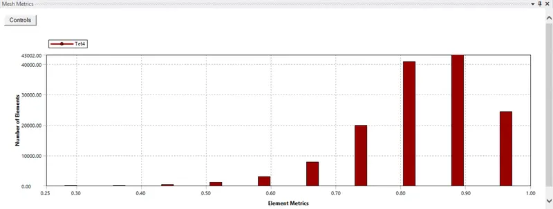
and the number of elements and nodes :

After creating the Mesh file, we name the geometry for the further use

1. Inlet x (inlet where the hot air come from)

2. Inlet y (inlet where the cold air come from)

3. The walls

4. Outlet

After updating the mesh file we go to the solution part.

Solution

SETUP	K-epsilon
Solver Type	Pressure Based
Velocity Formulation	Absolute
Time	Steady
Steady
Viscous Model	Realizable k-epsilon with standard wall function
Material	Fluid type: Air
Cell zones Volume_volume	Fluid type: Air
Boundaries	Inlet x (velocity inlet) Velocity Magnitude 3m/s Temperature – 36 degrees c. Inlet y (velocity inlet) Velocity Magnitude 6m/s Temperature – 19 degrees c. Outlet x (Pressure outlet) Gauge Pressure – 0 pas. Walls – Stationary walls

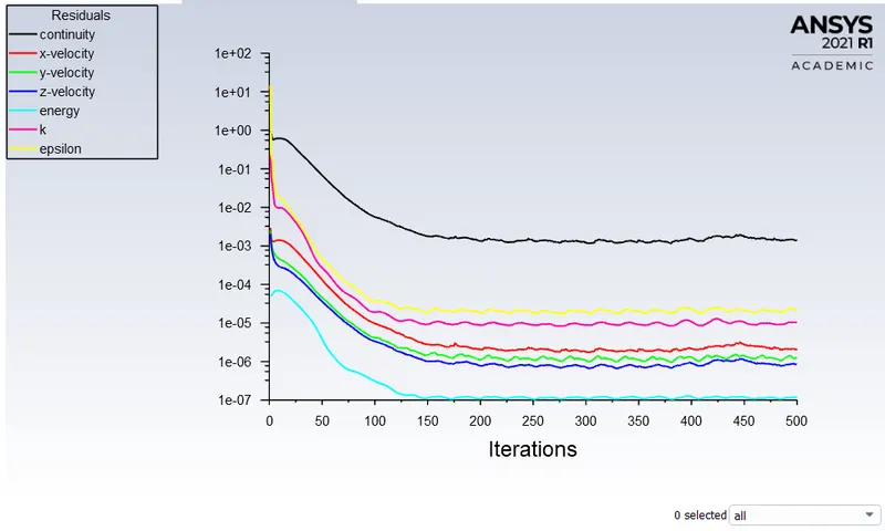
Residuals Plot

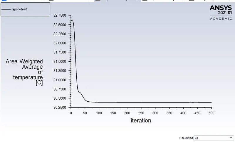
Average weighted area Plot to find the outlet Temperature

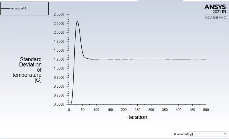
Standard Deviation Plot to find the Effectiveness of Mixing at the outlet

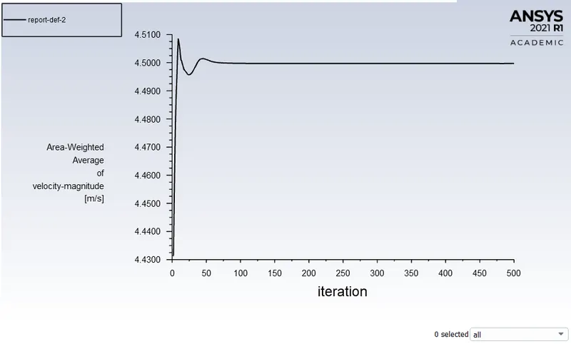
Average weighted area Plot to find the outlet Velocity

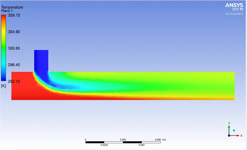
Counter Plot

1)For Temperature distribution

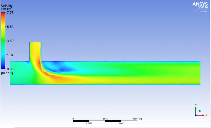
2)For Velocity Distribution

The flow of air in a pipe animation:

https://youtu.be/UEdhAHsoUgQ

CONCLUSION

• And as the length of the pipe increases the mixing has a lot of time and increases the temperature losing its main objective.

• In both cases of K-epsilon snd k-omega, k-epsilon has better results as we see in the residual plot these converge faster compared to k-omega
• From the above results, the meshing has to be improved. Which may give better results
• By doubling the chilled air velocity at the inlet results in better outlet mixing temperature which pretty much an acceptable result for us.