Week 1- Mixing Tee

QUESTION:

For this challenge, we have created two versions of the mixing tee. One of them is longer than the other.

Your job is to set up steady-state simulations to compare the mixing effectiveness when the hot inlet temperature is 360C & the Cold inlet is at 190C.

Use the k-epsilon and k-omega SST model for the first case and based on your judgment use the more suitable model for further cases. Giving the reason for choosing a suitable model is compulsory.

1. Case 1
• Short mixing tee with a hot inlet velocity of 3m/s.
• Momentum ratio of 2, 4.
2. Case 2
• Long mixing tee with a hot inlet velocity of 3m/s.
• Momentum ratio of 2, 4.

Momentum ratio = velocity at cold inlet/velocity at hot inlet

In a table, compare the following values from the 2 cases.

1. Cell count
2. Average outlet temperature
3. Number of iterations for convergence

Expected results:

1. Velocity and temperature contour plots on the cut planes along and across the pipe.
2. Velocity and temperature line plots along and across the length of the pipe.
3. Perform Mesh independent study for any one case.
4. Discuss the effect of length and momentum ratio on results.

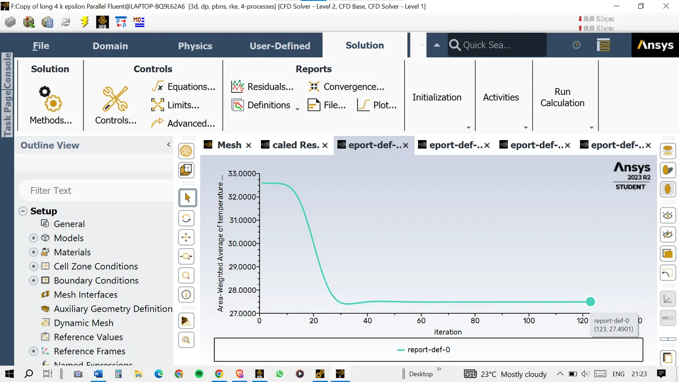
For each simulation, you need to show the convergence plot

ANSWER:

Simulation:https://drive.google.com/drive/folders/1QPSypgjQuwsIXlC8g-QftdcdSxZxW3TM?usp=sharing

Wordfile: https://docs.google.com/document/d/1EiSmEMbsJGw7BQXlgnL-Af6DllwLtHux/edit?usp=sharing&ouid=109197990435765605826&rtpof=true&sd=true

AIM:

This study aims to compare the mixing effectiveness in two versions of a mixing tee with different lengths. Steady-state simulations will be conducted using the k-epsilon and k-omega SST turbulence models for the first case, and the more suitable model will be selected for subsequent cases. The simulations will investigate the impact of varying momentum ratios (2 and 4) on a short and a long mixing tee, both with a hot inlet temperature of 36°C and a cold inlet temperature of 19°C. The study aims to analyze key parameters, including cell count, average outlet temperature, convergence behavior, and the influence of length and momentum ratio on results, providing visualizations and insights into the flow characteristics.

INTRODUCTION:

In this simulation study, we aim to investigate the mixing effectiveness in two versions of a mixing tee with different lengths. The mixing tee serves a critical role in industrial processes where fluids of contrasting temperatures are combined. Our focus is on comparing the performance of two turbulence models, k-epsilon and k-omega SST, in capturing the mixing characteristics under varying conditions.

Computational Fluid Dynamics (CFD):

Computational Fluid Dynamics (CFD) is a branch of fluid mechanics that uses numerical methods and algorithms to simulate the behavior of fluid flows. It involves the division of a fluid domain into small computational elements, called cells, and the solution of governing equations (such as the Navier-Stokes equations) to obtain a numerical approximation of the fluid flow. CFD has applications in various engineering fields, including aerodynamics, heat transfer, combustion, and chemical processes.

THEORY:

Mixing Tee in CFD:

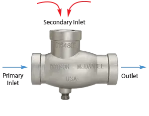
A mixing tee is a component commonly used in industrial processes where different fluid streams need to be combined. The behavior of fluid mixing in a tee is crucial in applications such as chemical reactors, pipelines, and HVAC systems. Computational Fluid Dynamics can be employed to analyze the flow patterns, turbulence, and mixing efficiency within a mixing tee.

In the context of Computational Fluid Dynamics (CFD) simulations for mixing tees, the choice of turbulence models, such as k-epsilon and k-omega SST, is crucial for accurately predicting turbulent flow behavior. Here's a brief overview of how these models are applied in the simulation of a mixing tee:

1. k-epsilon Turbulence Model:

· The k-epsilon model solves two transport equations, one for turbulent kinetic energy k and another for the rate of dissipation epsilon.

· It is widely used for its computational efficiency and is suitable for simulating a broad range of turbulent flows.

· In the context of a mixing tee, k-epsilon can provide insights into turbulence intensity and energy dissipation, influencing mixing patterns.

2. k-omega SST Turbulence Model:

· The k-omega SST model is an extension that combines elements of both k-epsilon and k-omega models.

· It employs the k-omega model in the near-wall region, ensuring better accuracy in predicting near-wall turbulence effects.

· Away from the wall, it transitions to a k-epsilon formulation, maintaining computational efficiency and versatility.

· In a mixing tee, k-omega SST can offer improved accuracy, especially in regions with adverse pressure gradients and separation.

Importance in Practical Applications:

1. Design Optimization:

CFD simulations of mixing tees with turbulence models help optimize the design for efficient mixing. Engineers can assess different geometries, inlet conditions, and momentum ratios to achieve desired mixing characteristics.

2. Heat Transfer Analysis:

In applications involving temperature-sensitive processes, such as chemical reactions, HVAC systems, or industrial heat exchangers, CFD with turbulence models aids in understanding heat transfer patterns within the mixing tee.

3. Energy Efficiency:

Efficient mixing is often crucial for processes where energy conservation is a priority. CFD simulations enable engineers to identify design modifications that enhance energy efficiency.

4. Scale-Up Considerations:

Understanding the performance of a mixing tee in CFD simulations allows engineers to extrapolate findings for different scales, facilitating the design and analysis of larger systems.

5. Troubleshooting and Optimization:

CFD provides a virtual environment to troubleshoot potential issues in mixing tee performance. Engineers can iteratively optimize designs before physical prototypes are built, saving time and resources.

Solving and Modelling Approach:

Geometry Setup > Turbulence Model Selection > Momentum Ratio Variation > Simulation Settings > Post-Processing > Convergence Analysis > Results Discussion

v We will use this approach for both the cases and sub-cases.

CASE 1à MR-2 à K-EPSILON Vs K-OMEGA

MR-4 à SELECTED TURBULENCE MODEL

CASE2à MR-2 à SELECTED TURBULENCE MODEL

MR-4 à SELECTED TURBULENCE MODEL

Case1: Short Mixing Tee

Case 1.1: Momentum Ratio=2

In this case, we will set the steady-state simulation with both the k-epsilon and k-omega SST model, and after the result, I will go with the model that gives the best results to the application.

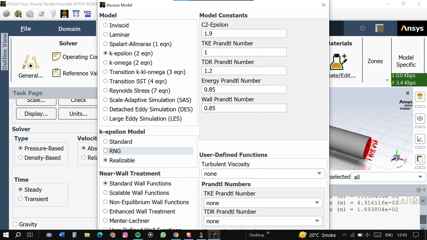
K-epsilon(Realizable)

Open the Ansys workbench and drag and drop the fluid flow (fluent) into the schematic window.

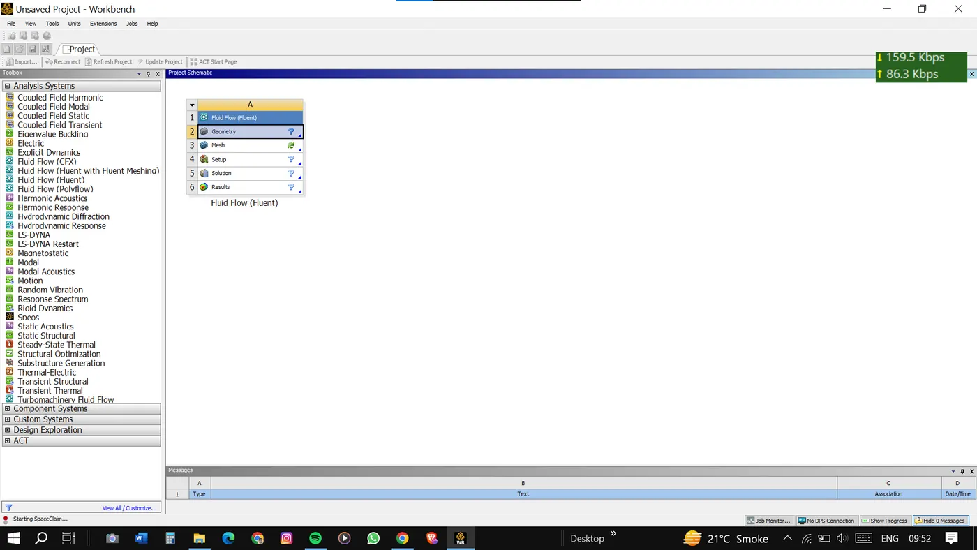
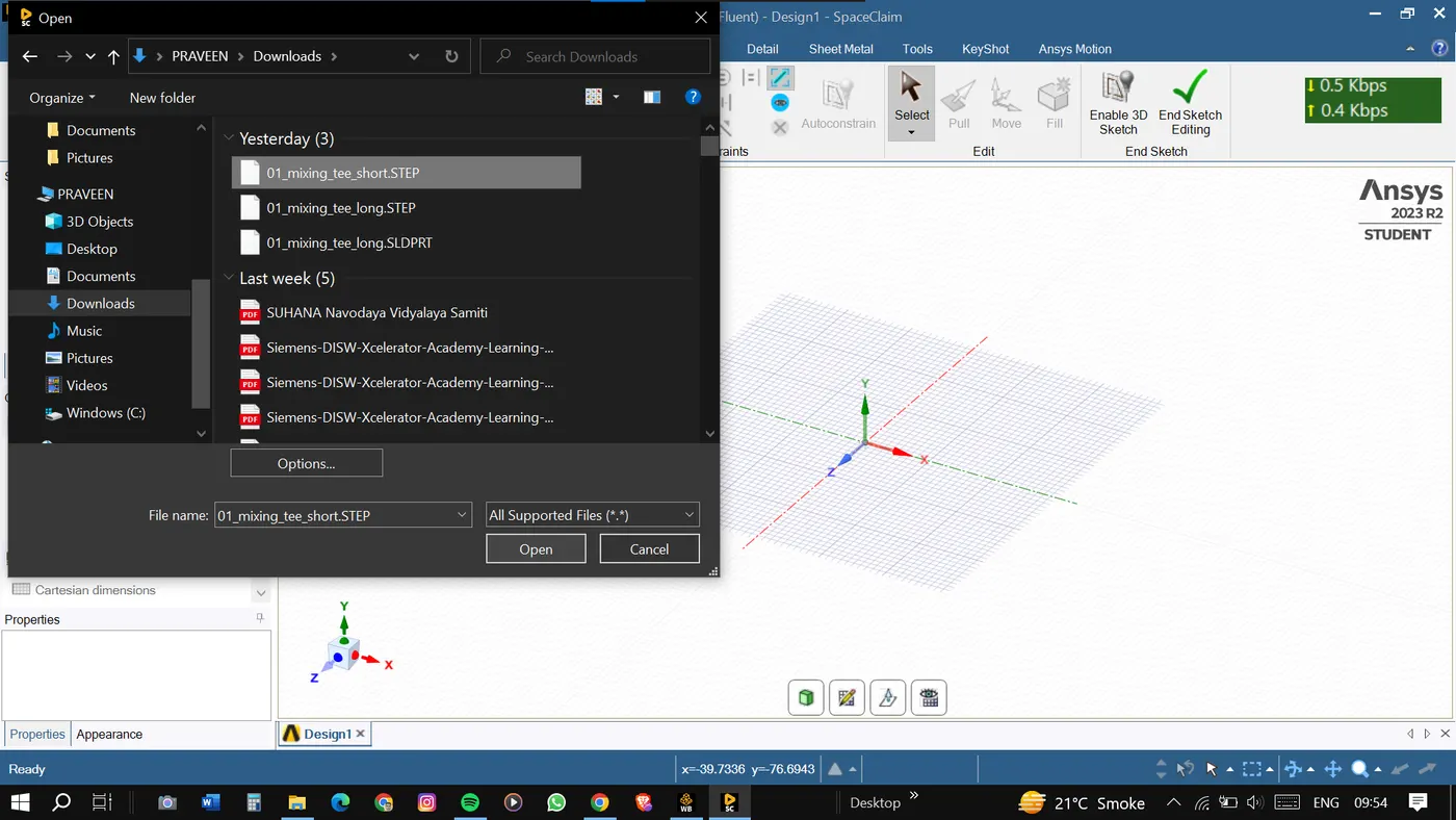
Double-click the geometry to open the SpaceClaim to set up the geometry for the simulation.

Open the model in the space claim.

Geometry Setup :

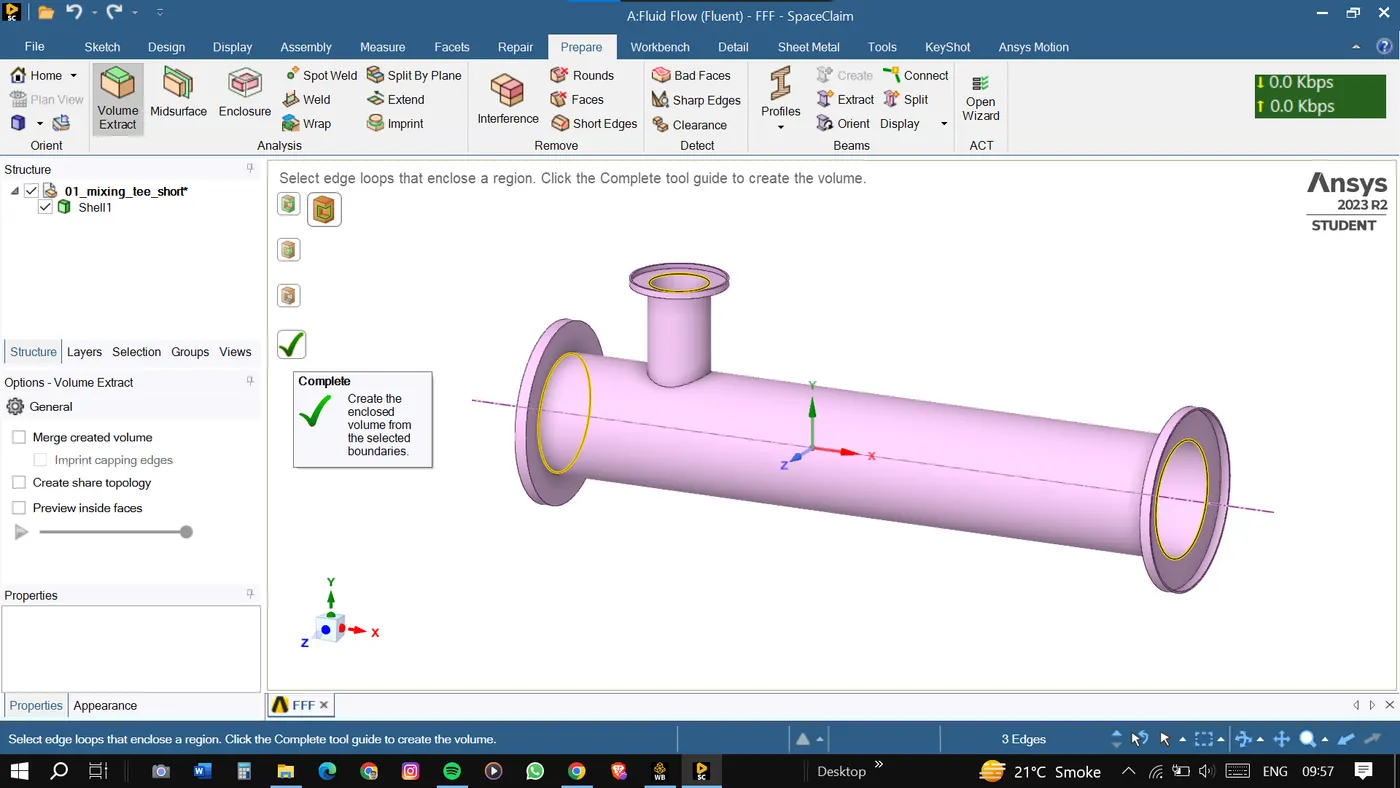
Once the model is open go to the prepare>>volume extract and then select the edges of the geometry from which the volume is to be extracted. And finally, click on the complete option to extract the fluid volume.

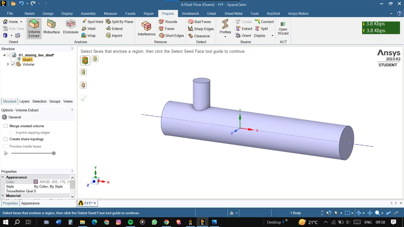
Once the volume is extracted, close the space claim and open the meshing.

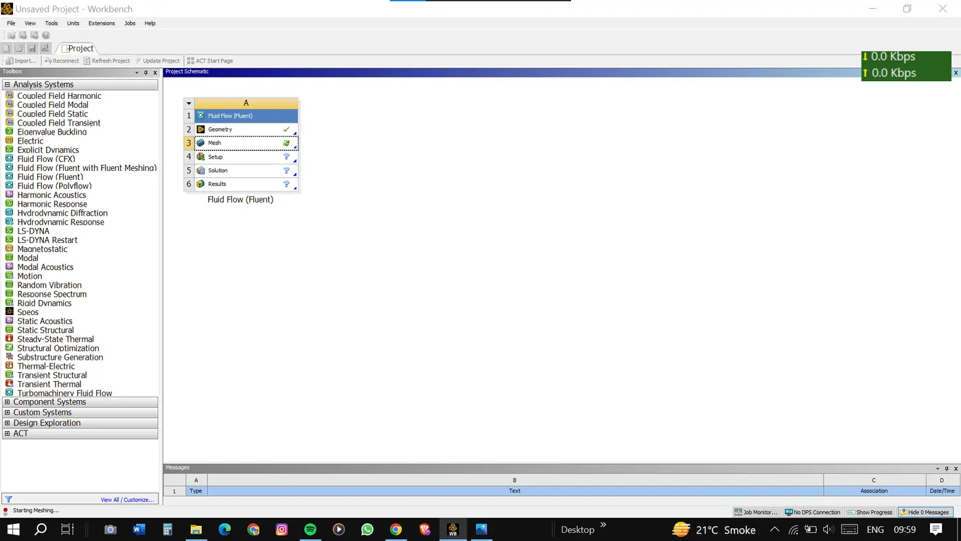
The things will be automatically saved and once we double-click the meshing module the geometry will be automatically loaded.

Meshing :

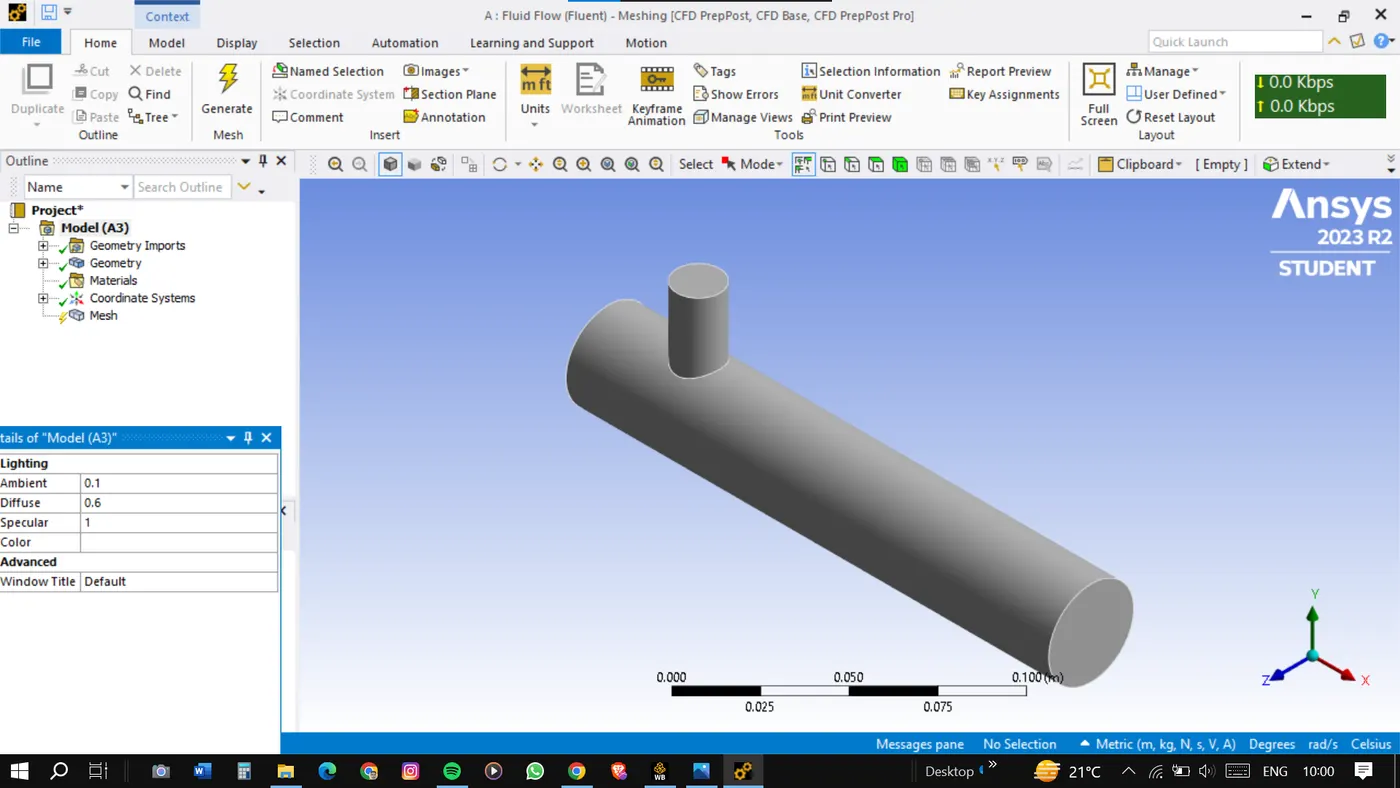
Once the model is loaded, create the boundaries for the simulation.

Select the face press N for named selection and enter the name for the inlet outlet and walls.

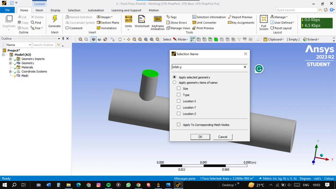
Then go for the meshing with the very basic options.

Right-click on the mesh and then click on the generated mesh.

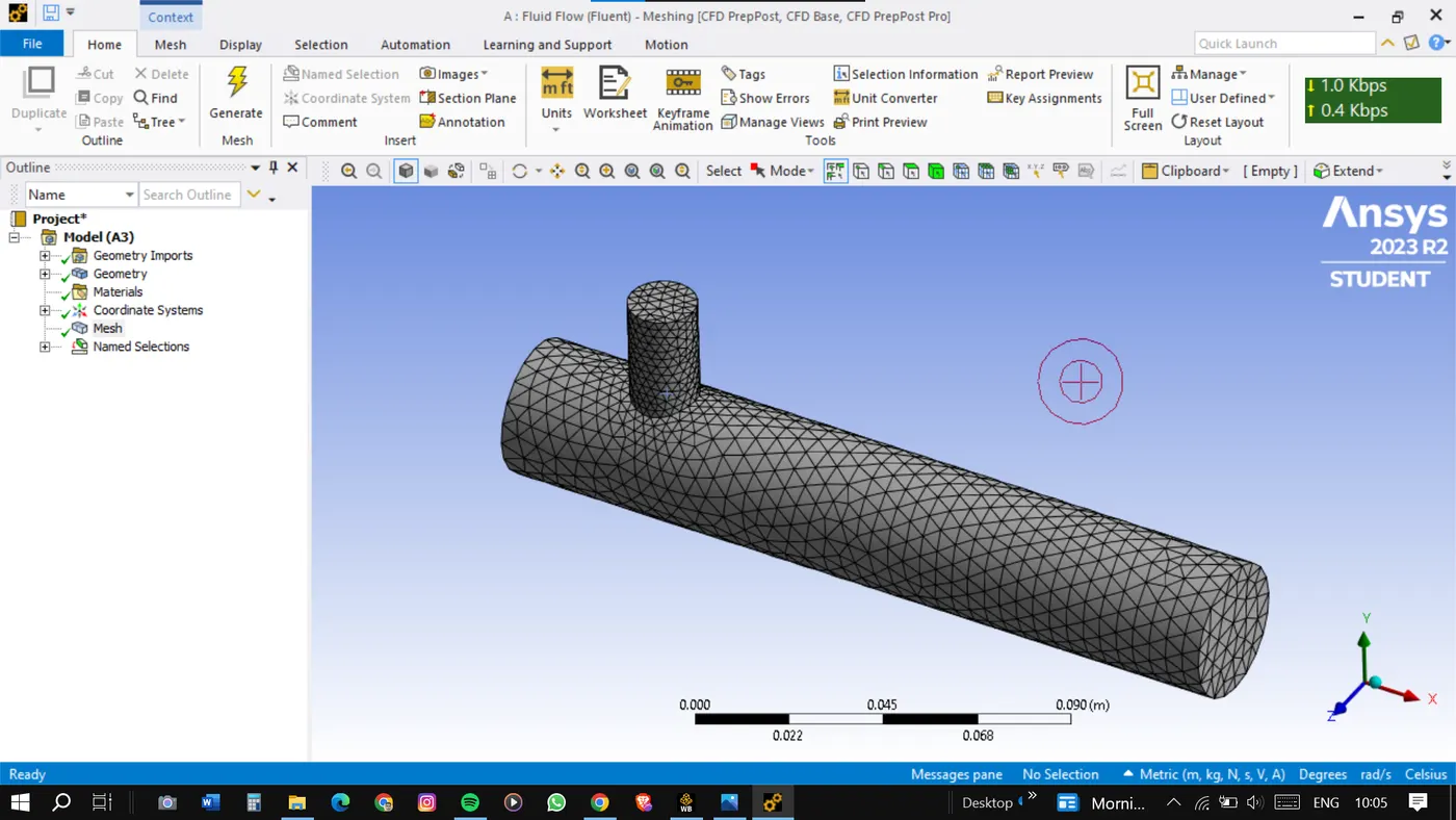
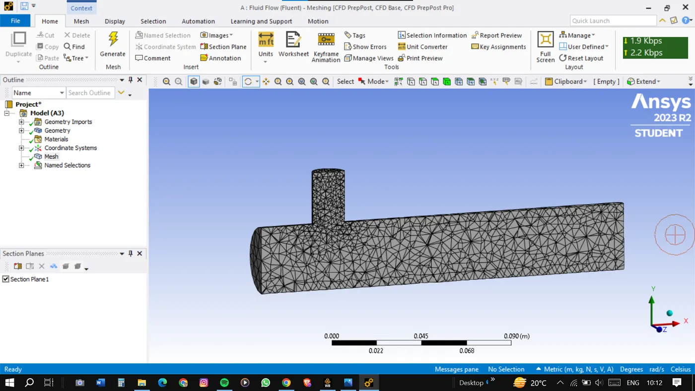
To analyze the mesh in the section view click on the section plane button and drag a line to cut the section.

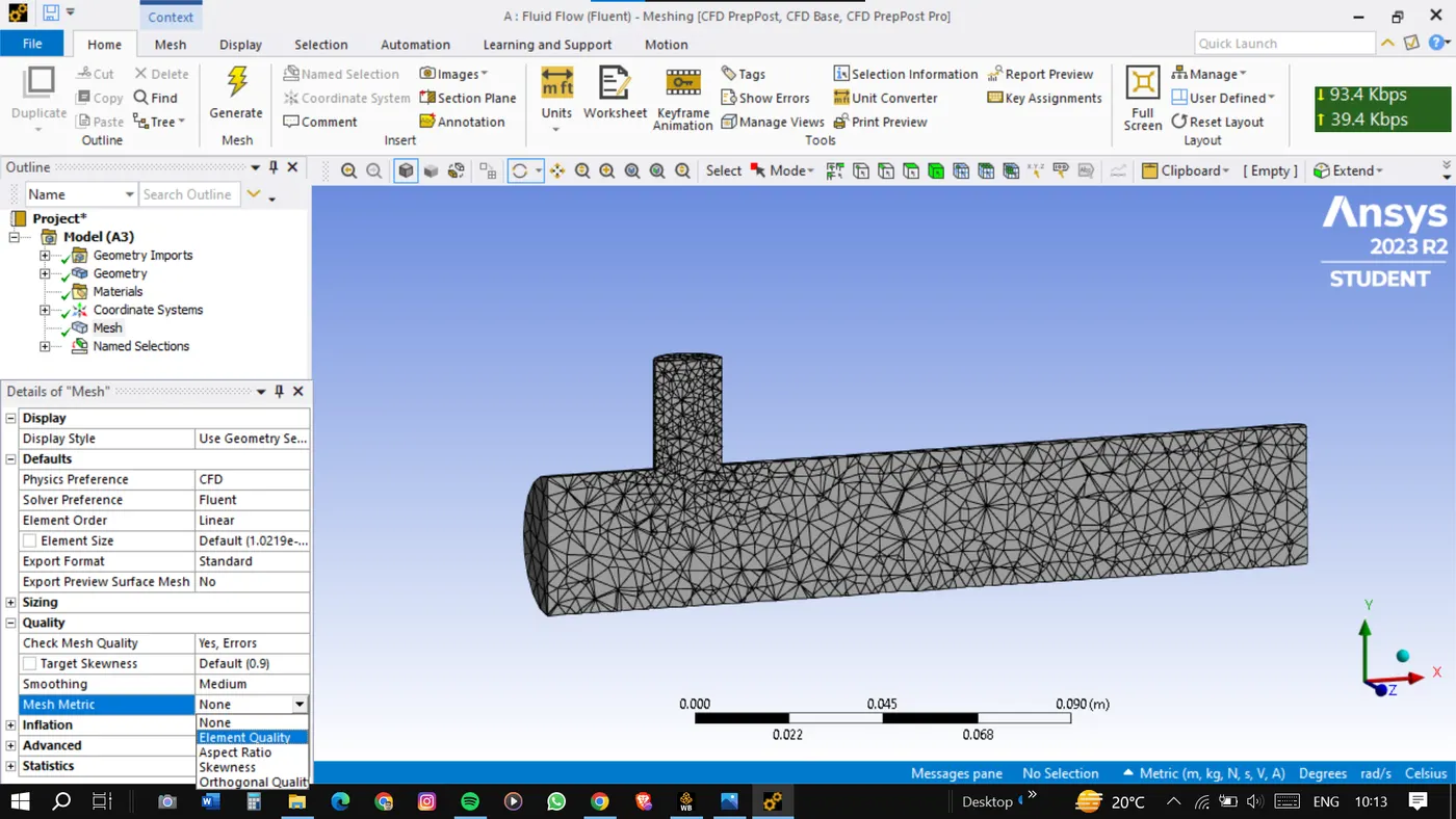
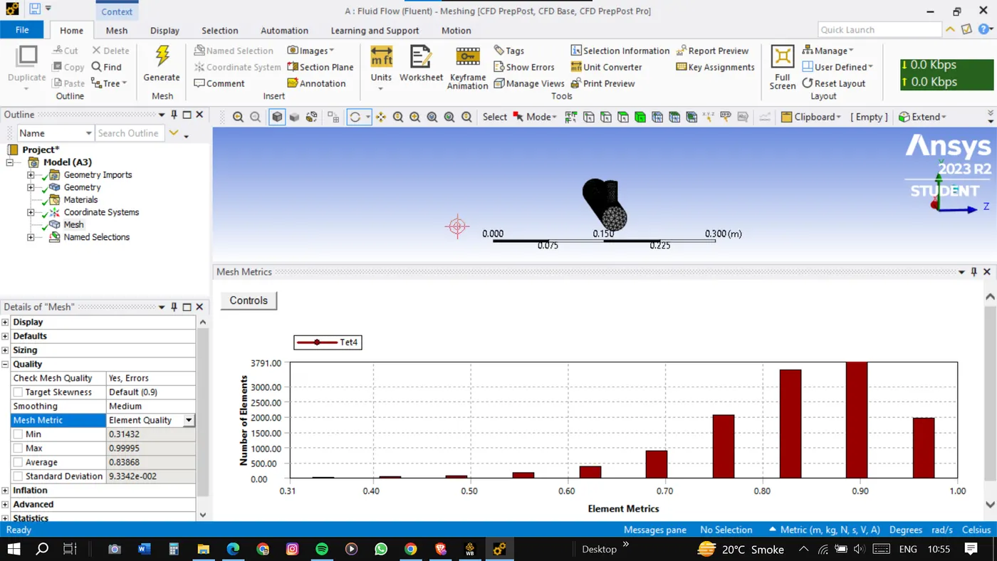
To check the element quality select the element quality for mesh metric and we will get the graph for the element quality.

It should not be less than 5% but in our case, it's 31% minimum and it's good to go.

Now close this and open the ansys fluent by clicking on the setup.

Fluent setup:

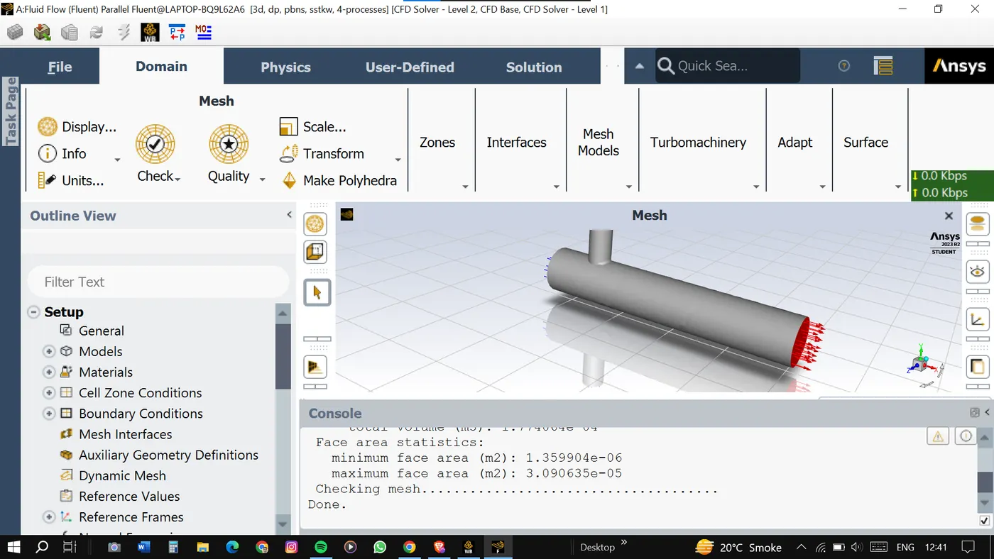
First of all, check the mesh quality by clicking on check.

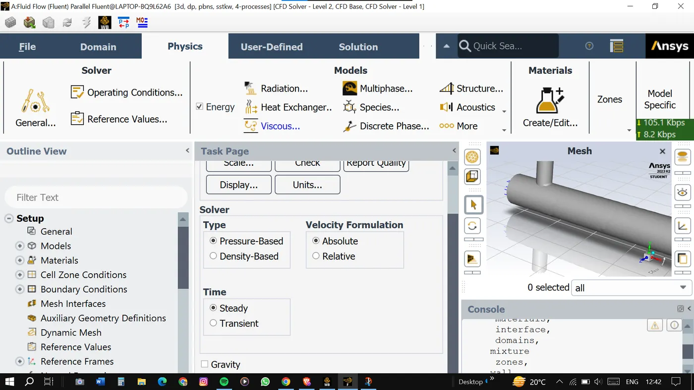
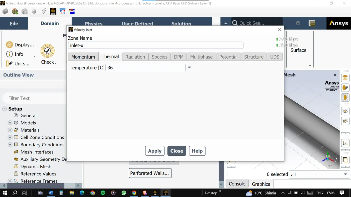
And setting up the physics for the case shown in the images below.

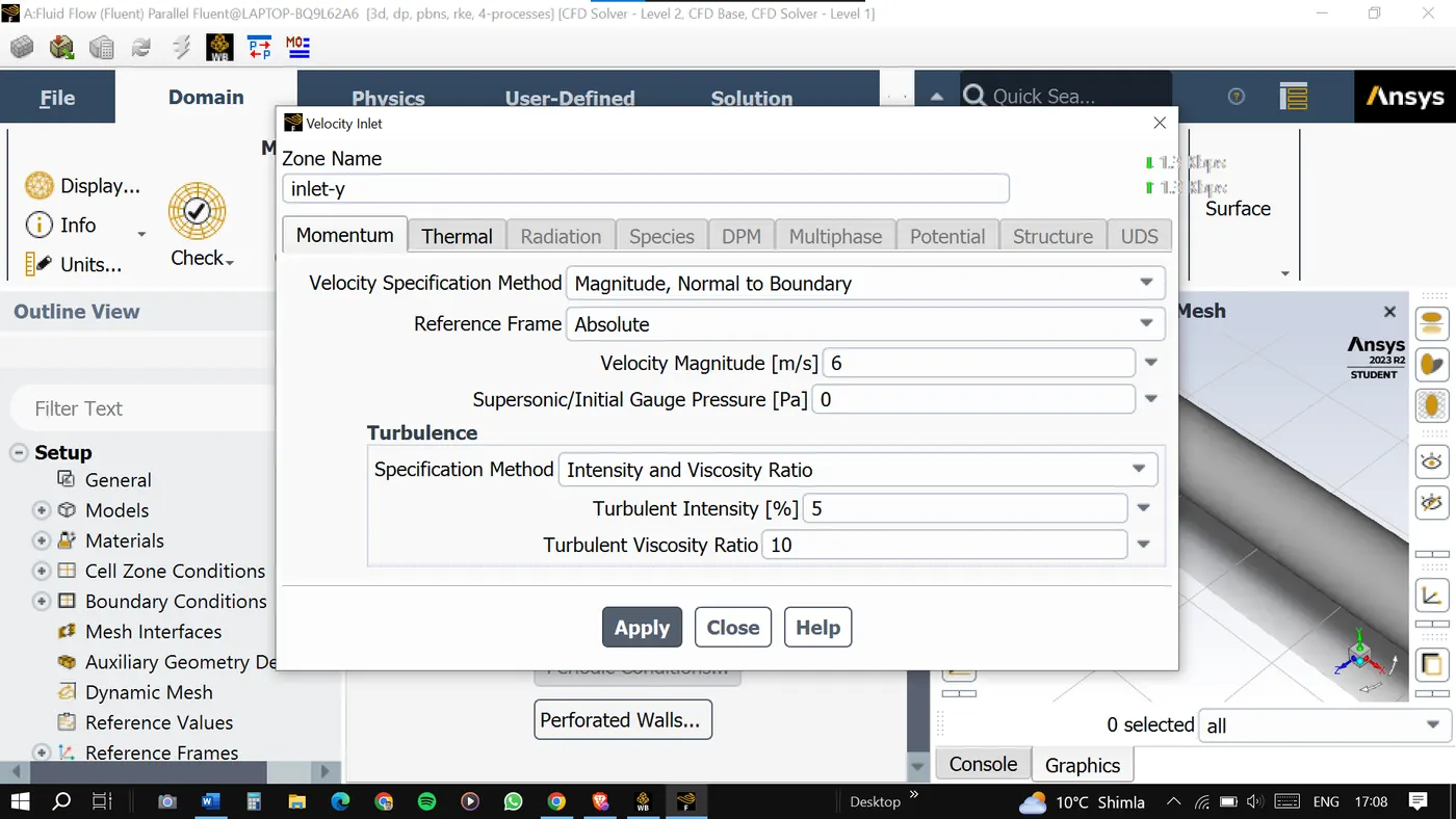
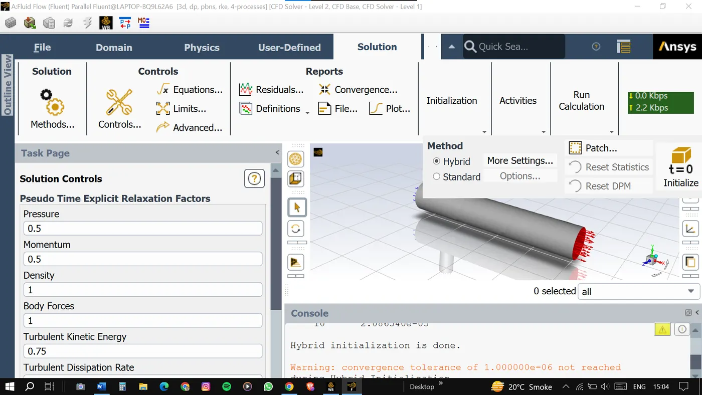
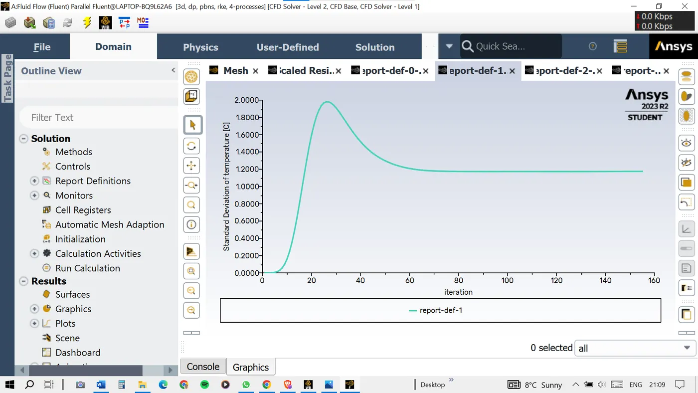
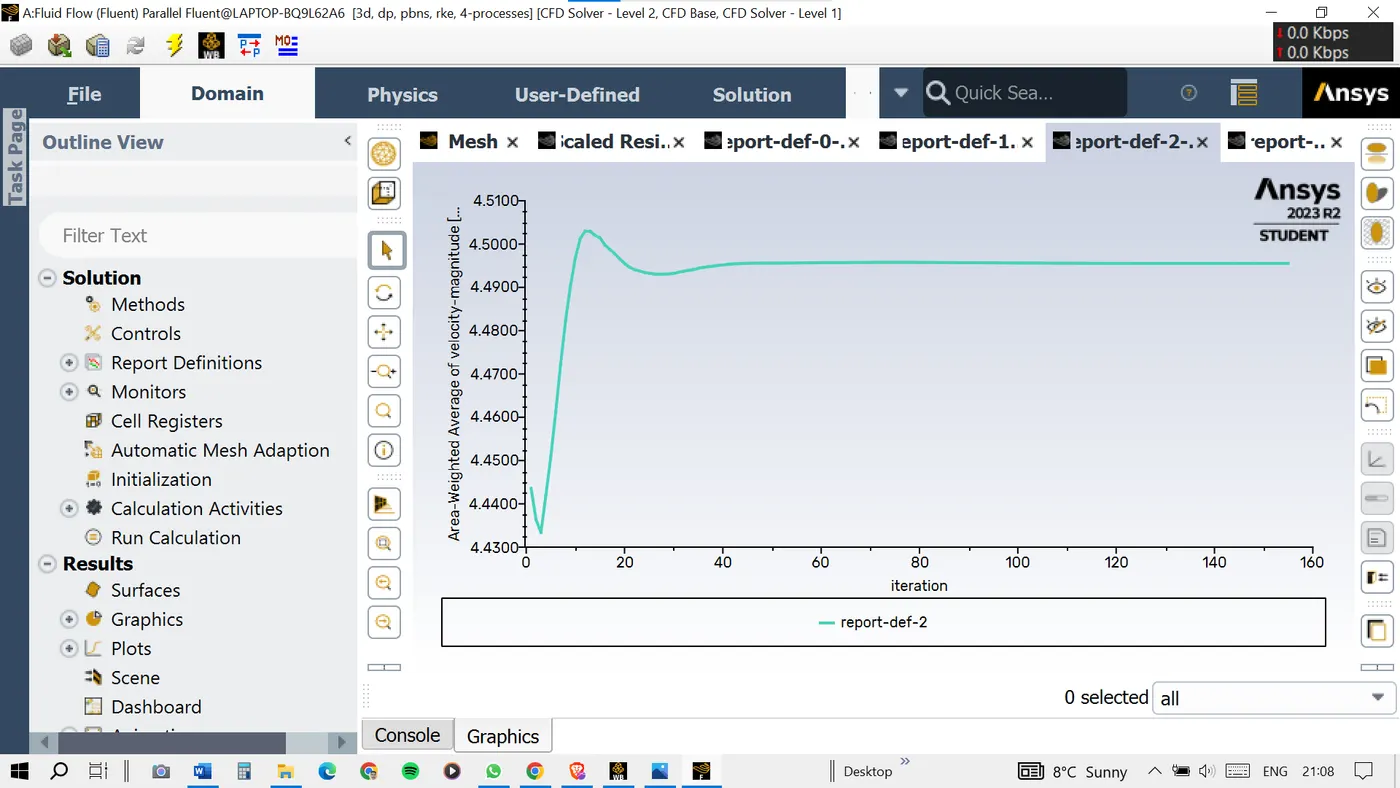
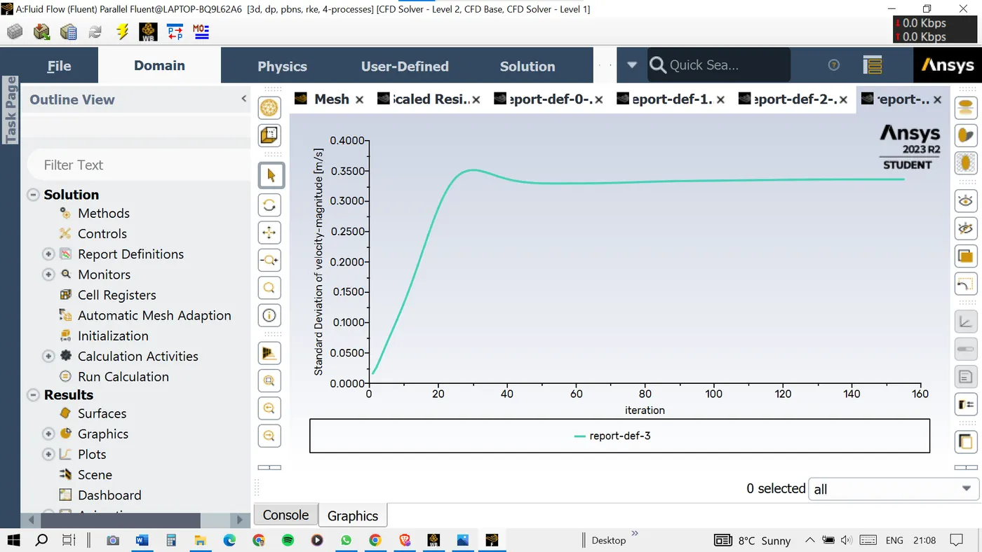
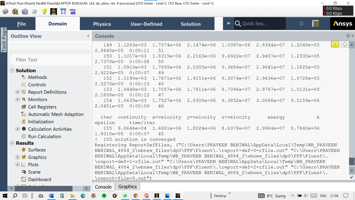
The plots for the k-epsilon model.

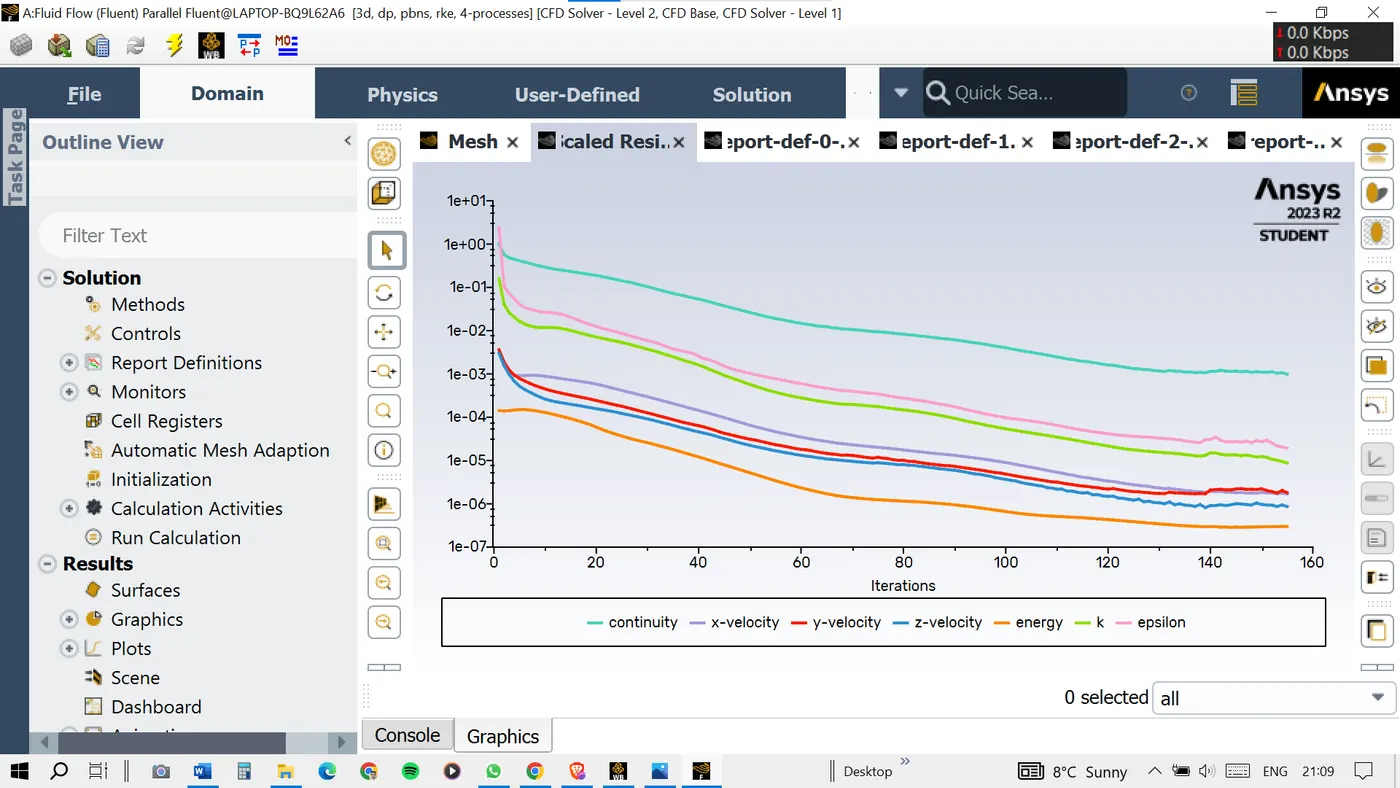
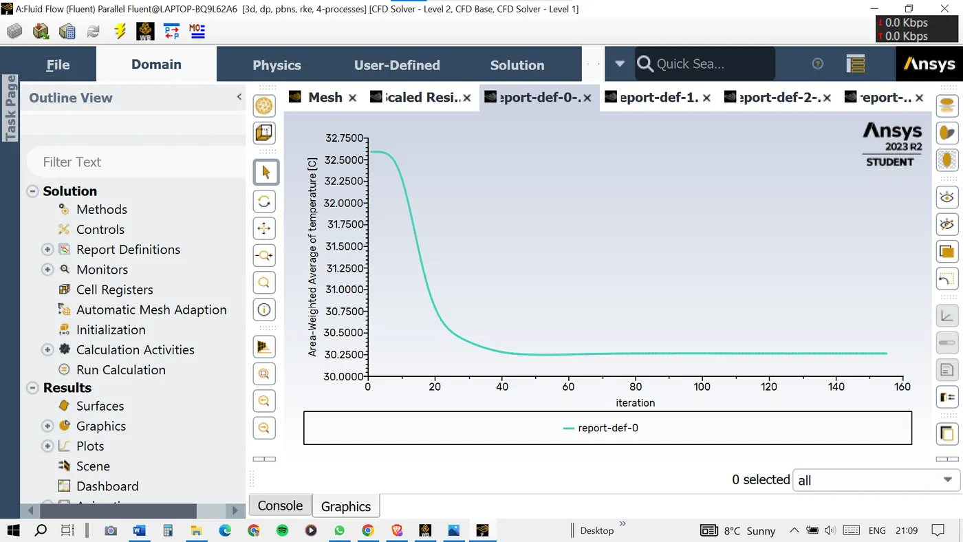
Once we get the plots for the simulation we can proceed with the results (CFD post).

CFD Post:

TEMPERATURE CONTOUR:

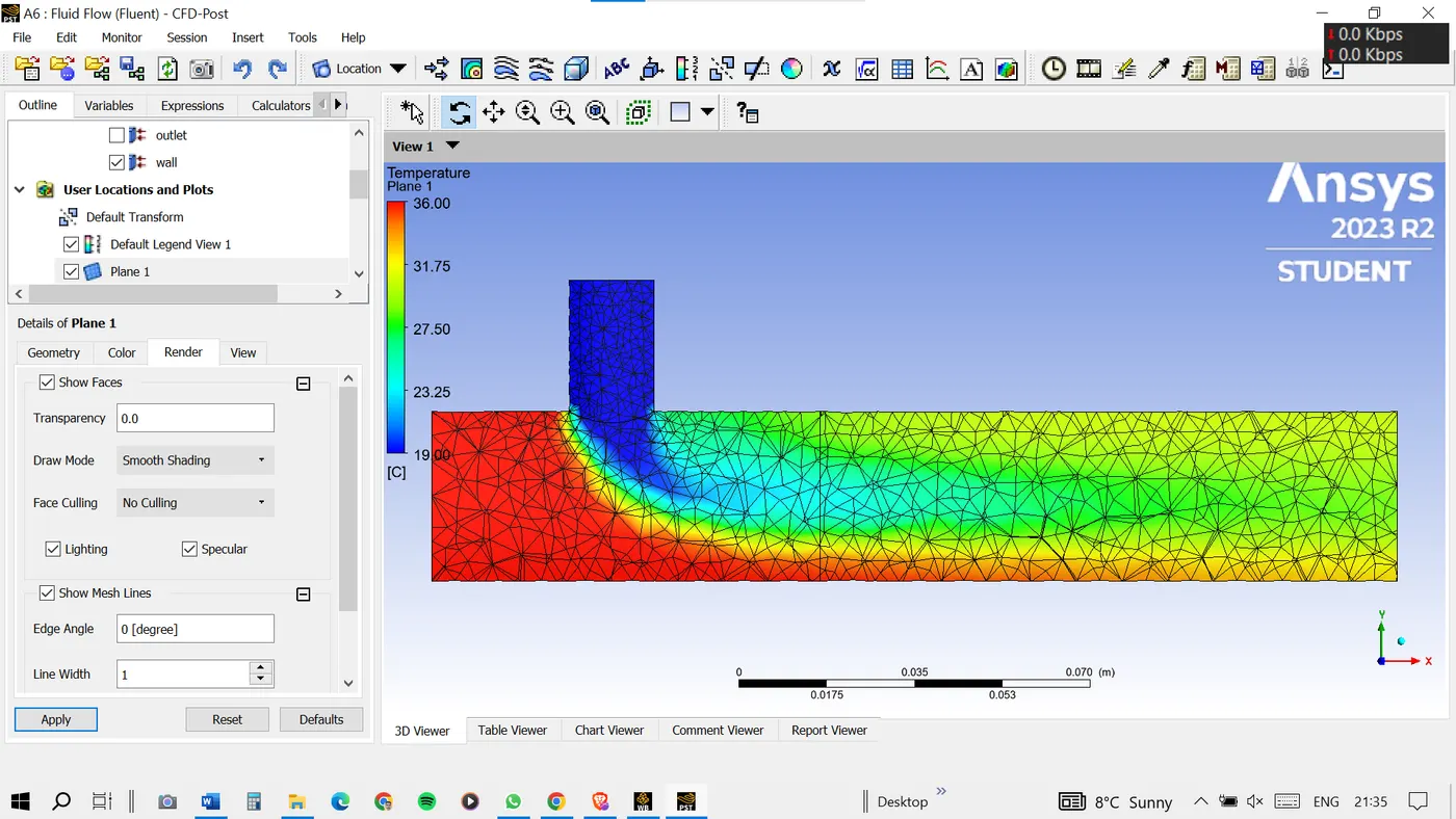
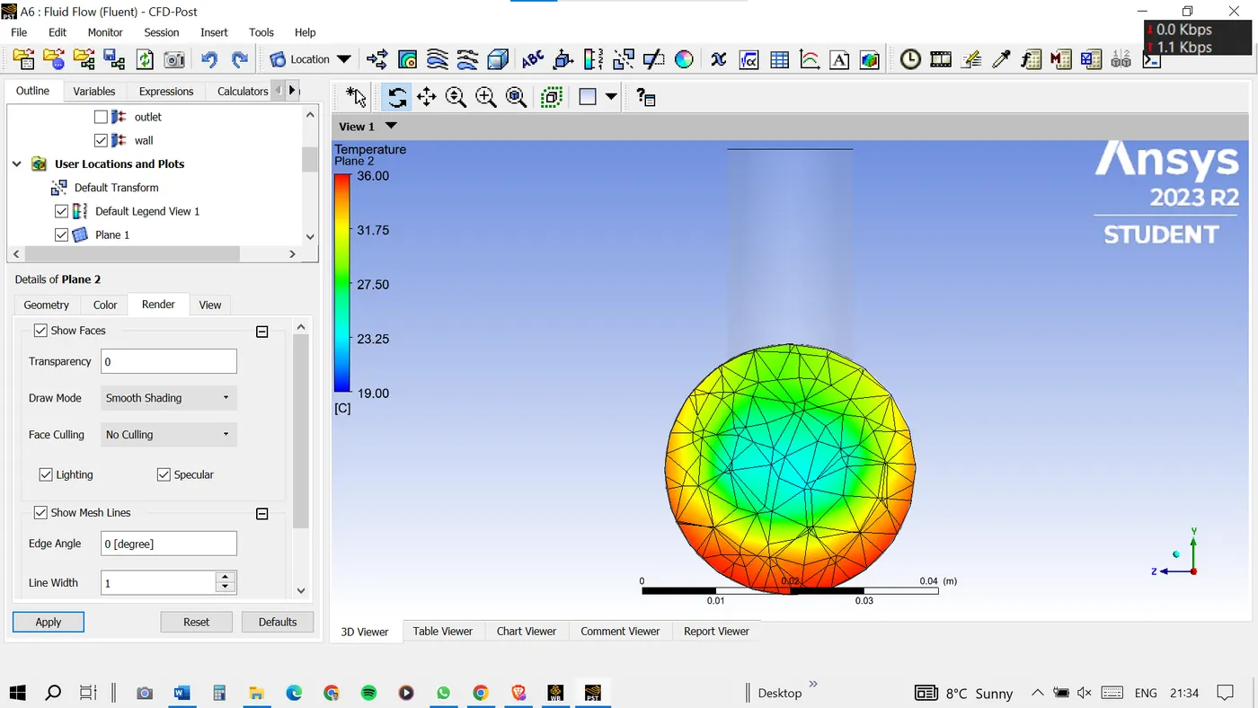
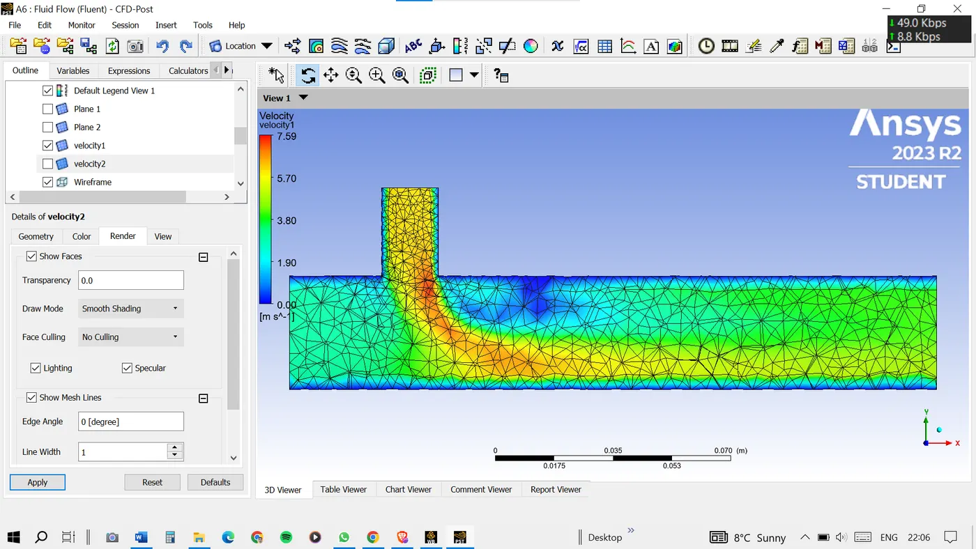
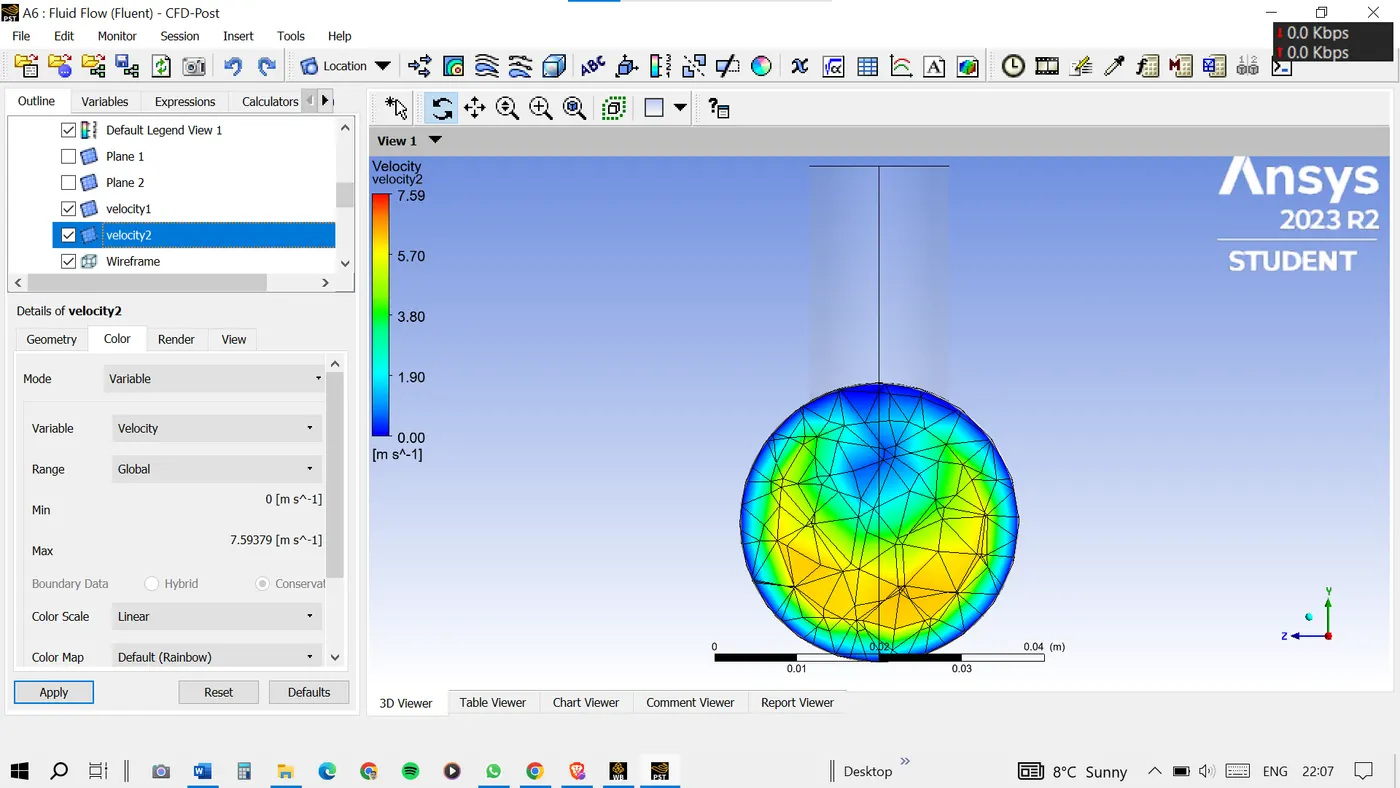
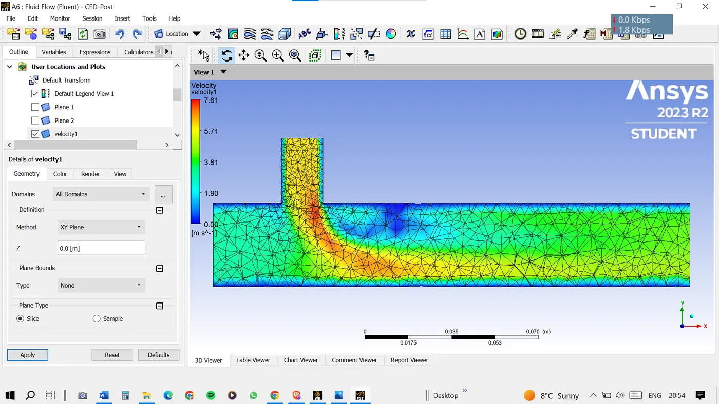
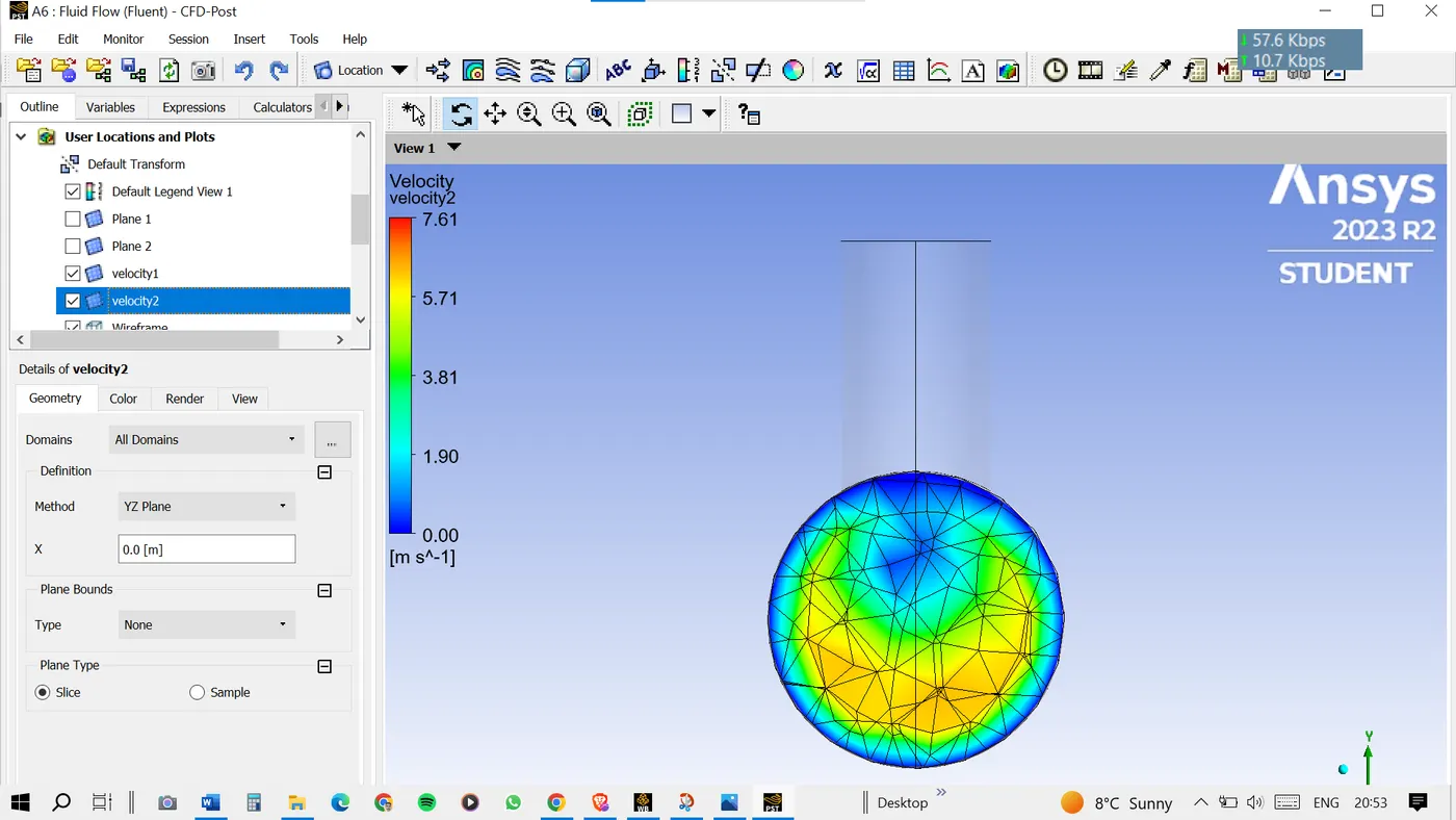
VELOCITY CONTOUR:

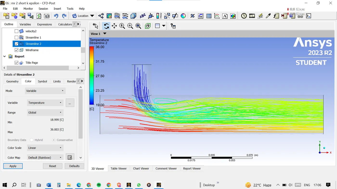
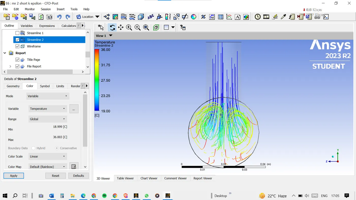
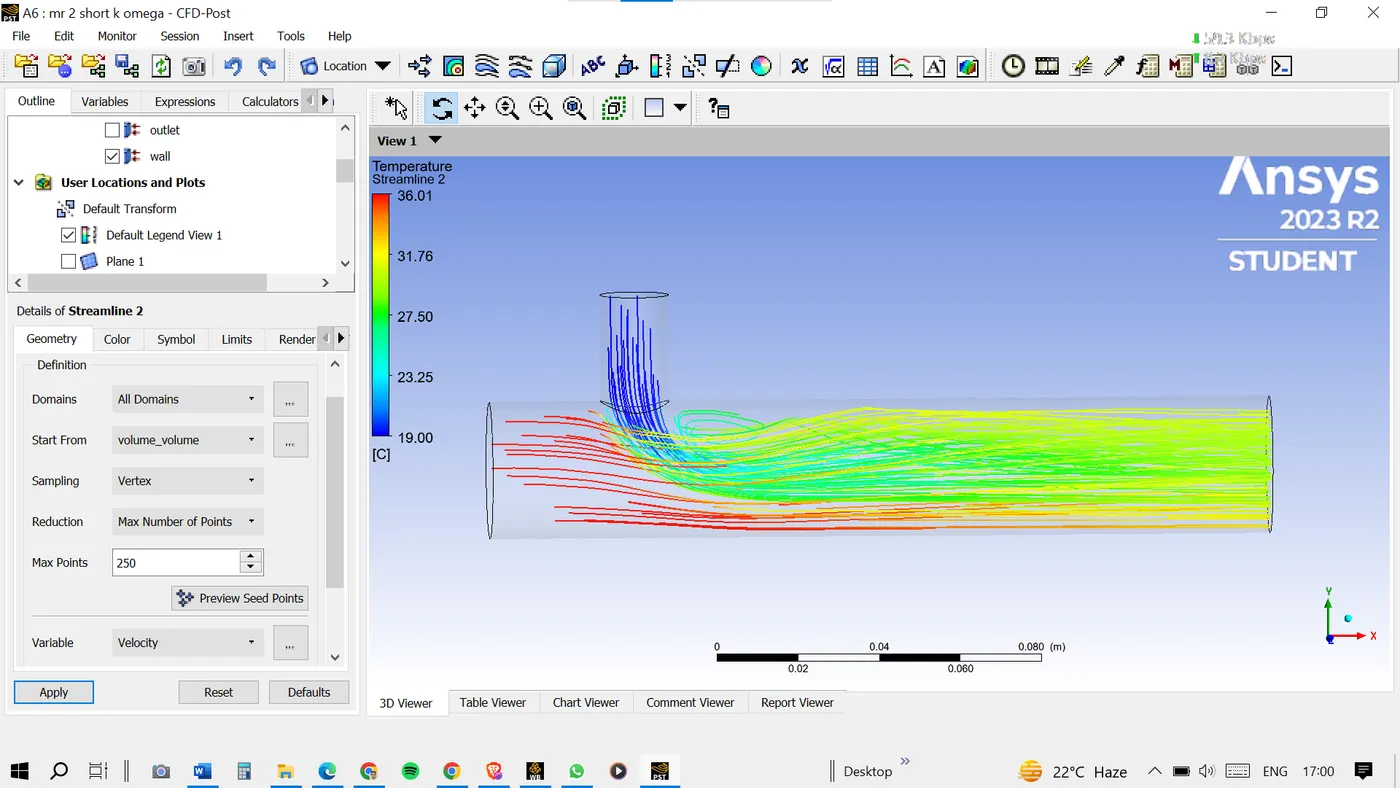
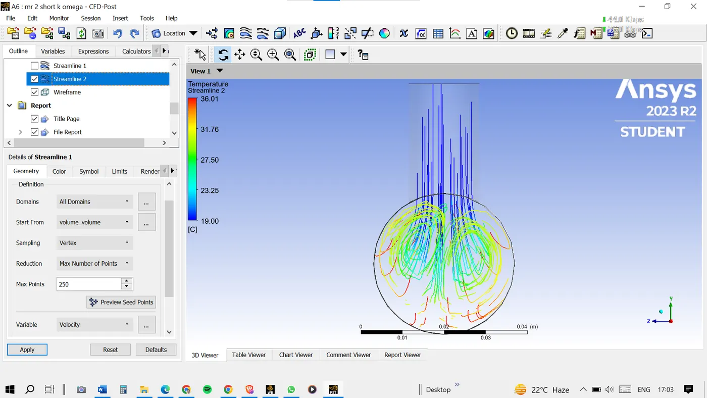
TEMPERATURE STREAMLINES:

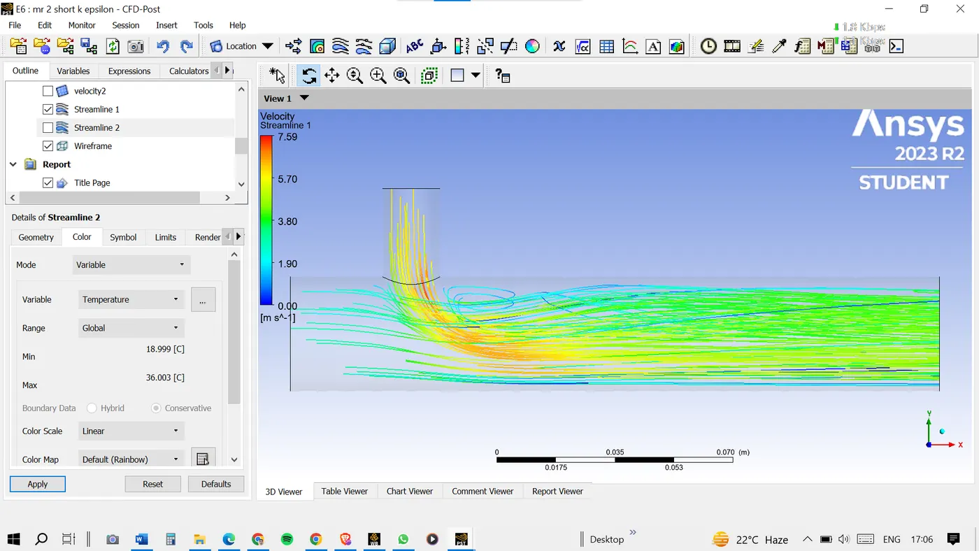
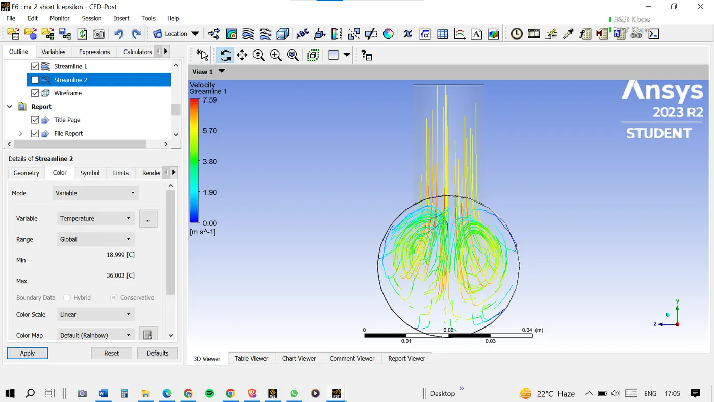
VELOCITY STREAMLINES:

Similarly, we will go for the k-omega. Only while selecting the turbulence model go with the k-omega (SST).

k-omega (SST)

Here also go with the same approach as for the above model only at the time of viscous model selection just select the k-omega SST model and further steps are also the same.

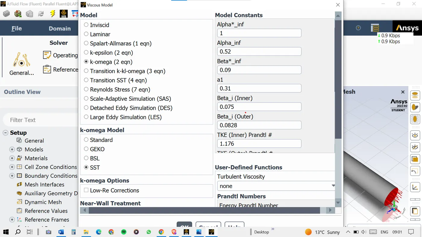
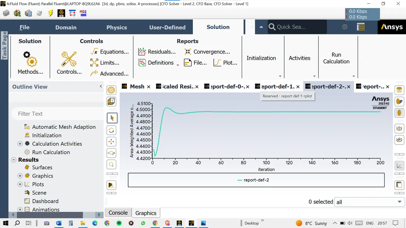
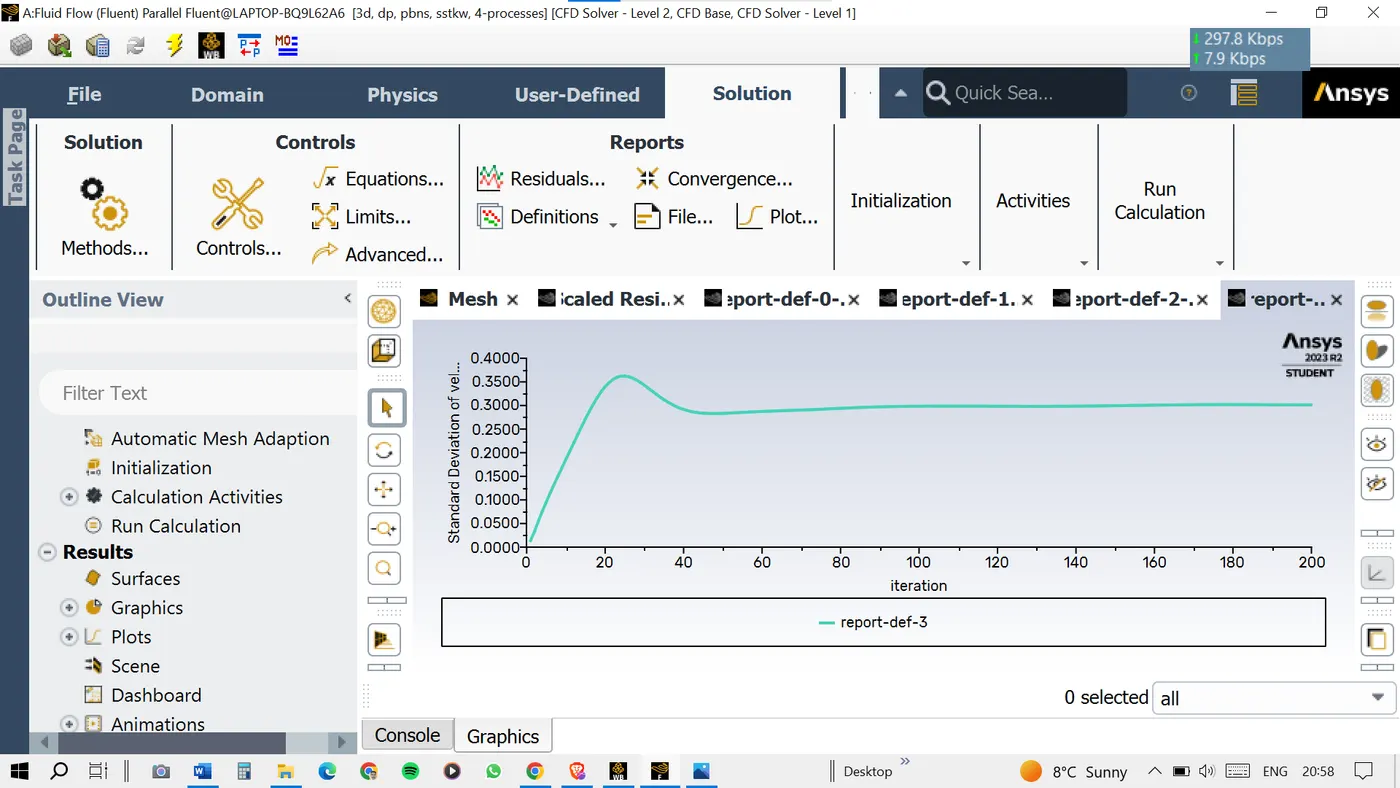
Plots for the K-omega SST model.

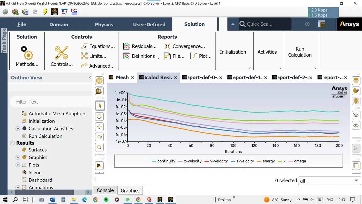
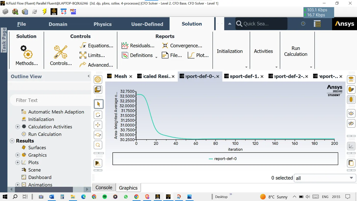
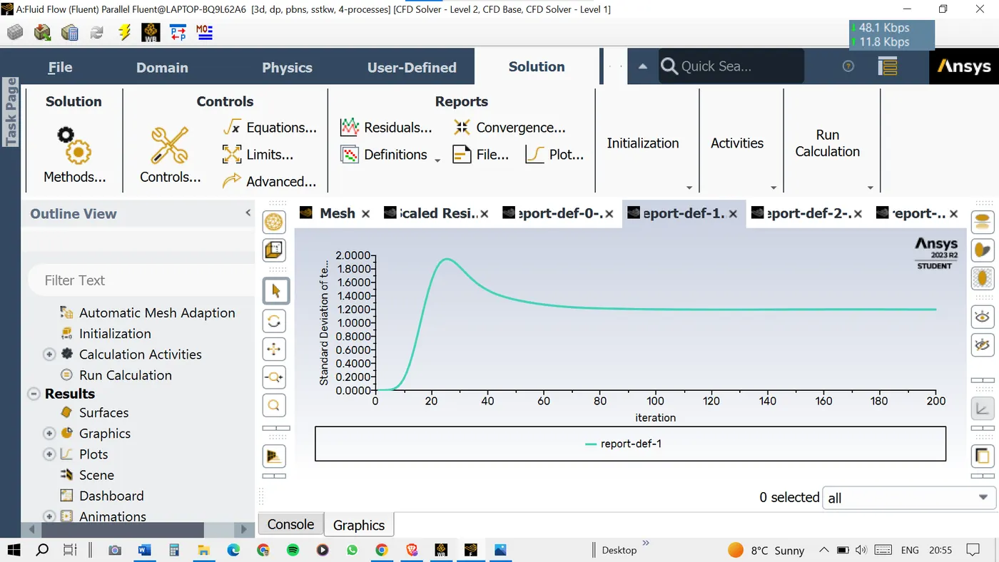
CFD Post :

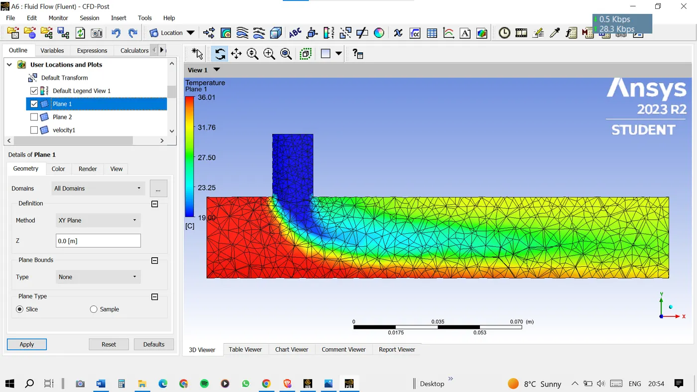
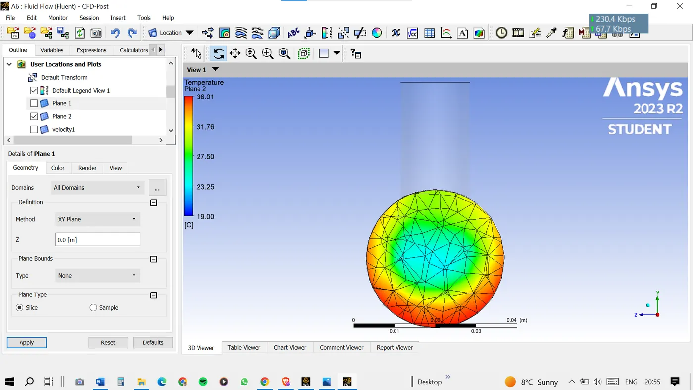
TEMPERATURE CONTOURS:

VELOCITY CONTOURS:

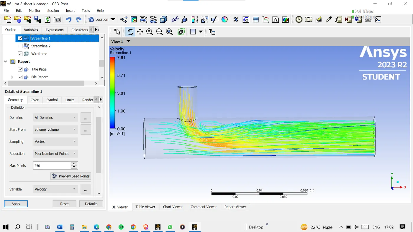
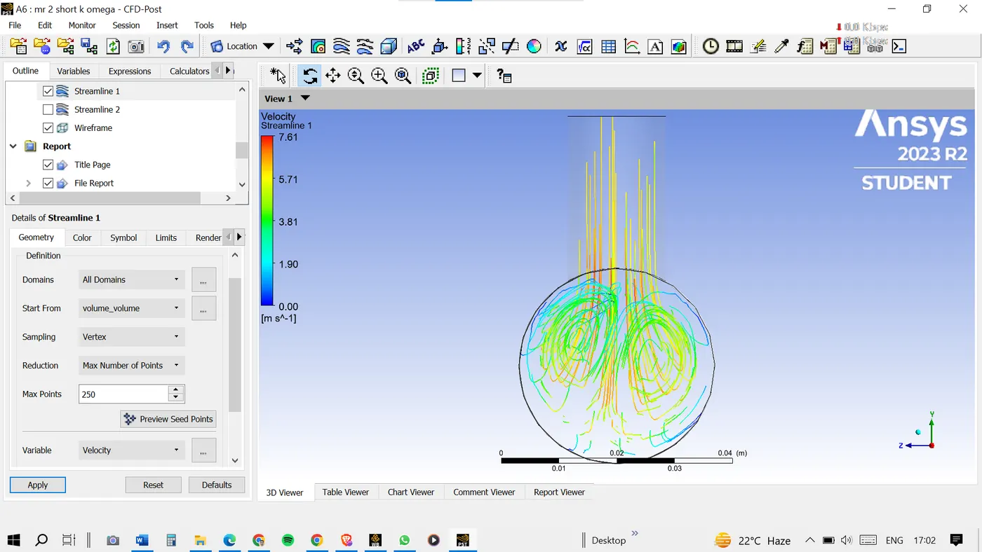
TEMPERATURE STREAMLINES:

VELOCITY STREAMLINES:

MODEL COMPARISON

It's time to compare the results of K-Epsilon and K-Omega SST models and choose the best fit for our other cases.

	K-epsilon	K-omega SST
No. of iterations to converge	155	200
Standard deviation	1.1755	1.1985
Average outlet temperature (C)	30.2635	30.2935

So after comparison, I have decided to use K-epsilon for further cases.

Reasons for choosing k epsilon are:

· It has taken less no of iterations to converge the solution because the K-epsilon Realizable model is simpler in formulation, involving fewer equations.

· Standard deviation is lower in the k- epsilon model. Hence more efficient.

· It has taken less time and given almost the same results.

· The K-epsilon Realizable model is generally computationally more efficient than the K-omega SST model, making it well-suited for simulations with large domains or when computational resources are limited.

· The K-epsilon Realizable model typically uses standard wall functions for near-wall treatment, which can be advantageous in cases where accurate predictions of near-wall behavior are not critical.

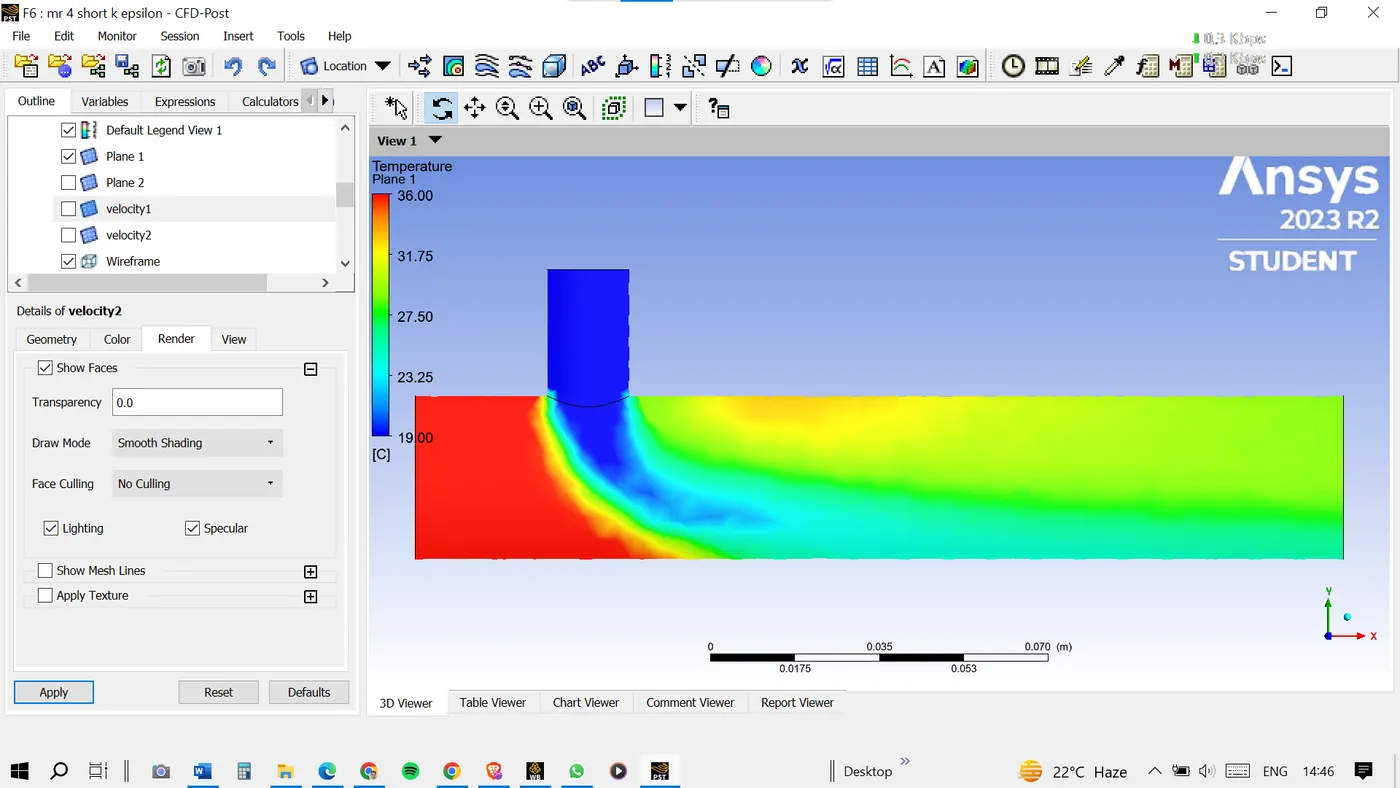
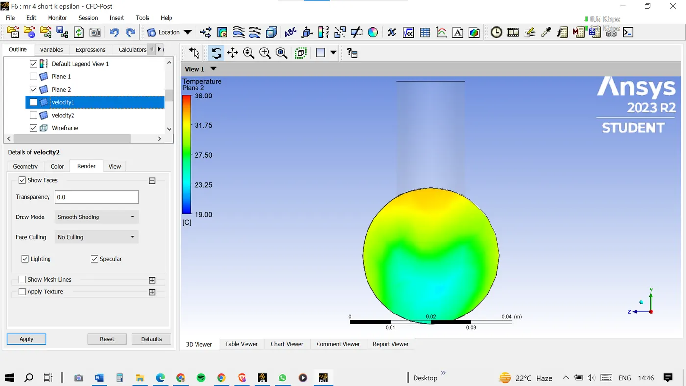
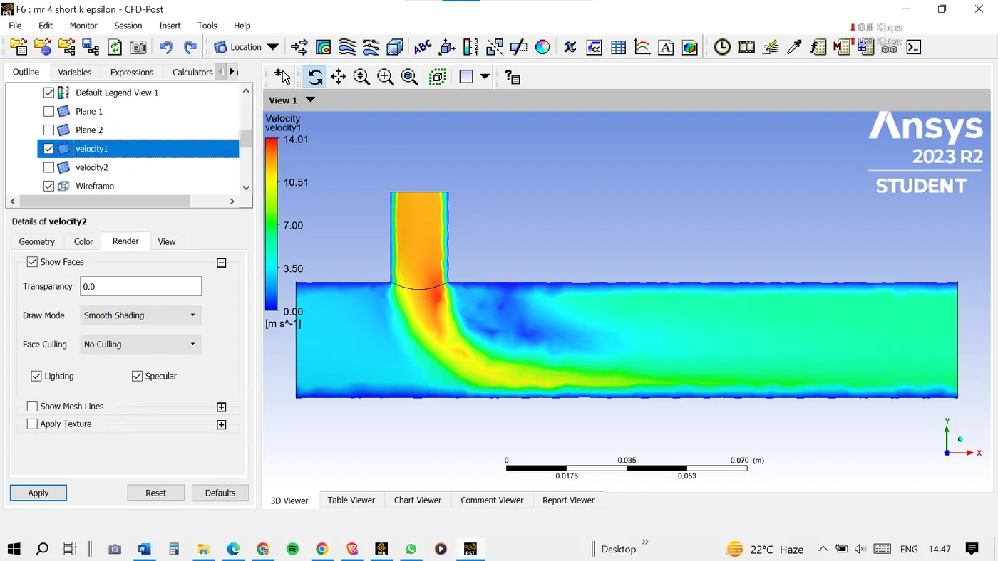
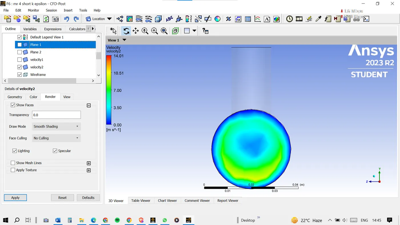
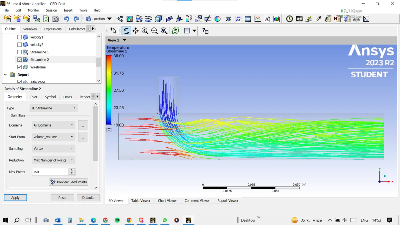
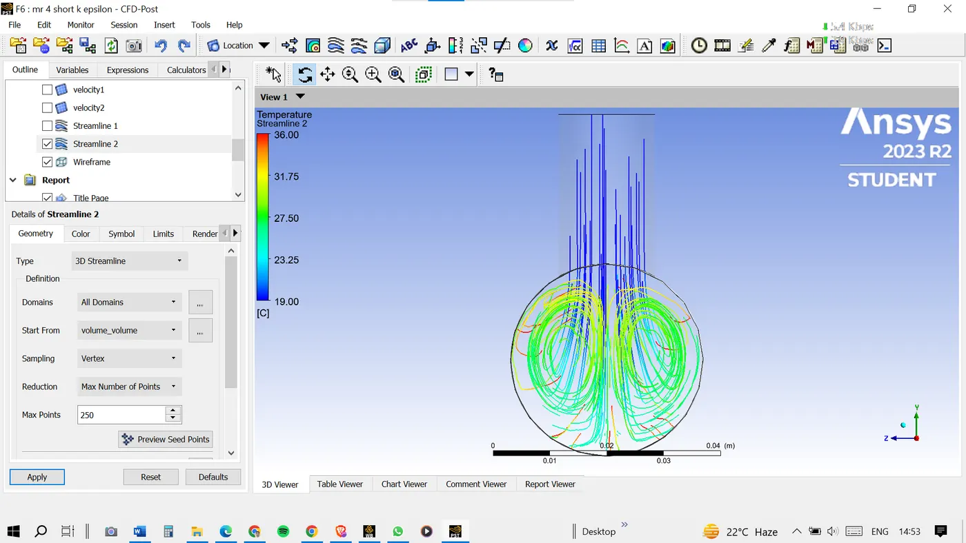
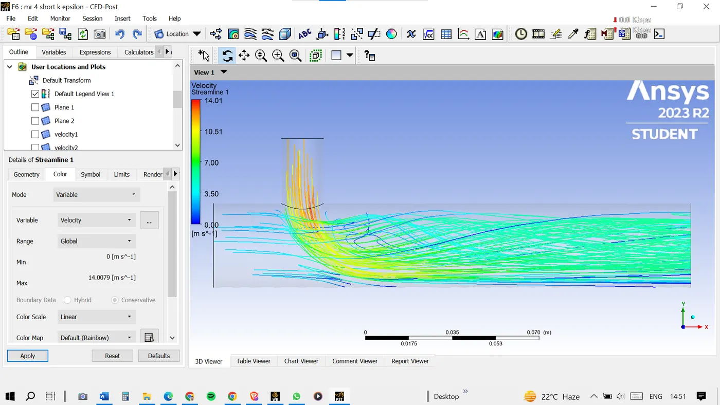
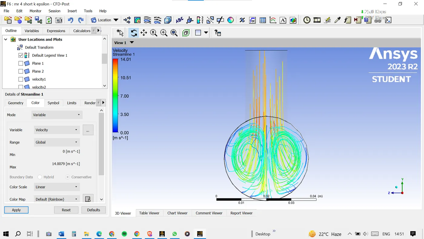
CASE 1.2: Momentum ratio=4

Plots for k-epsilon MR=4.

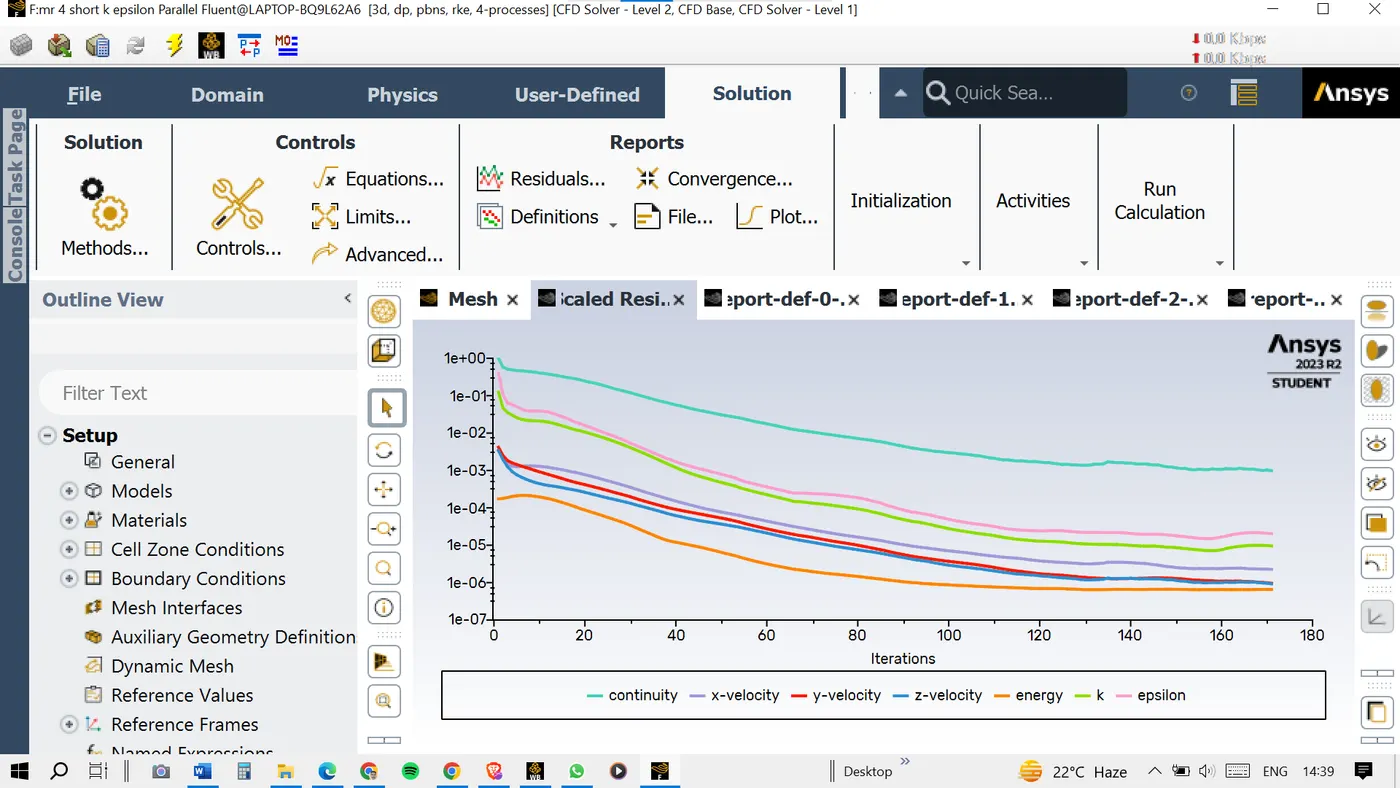
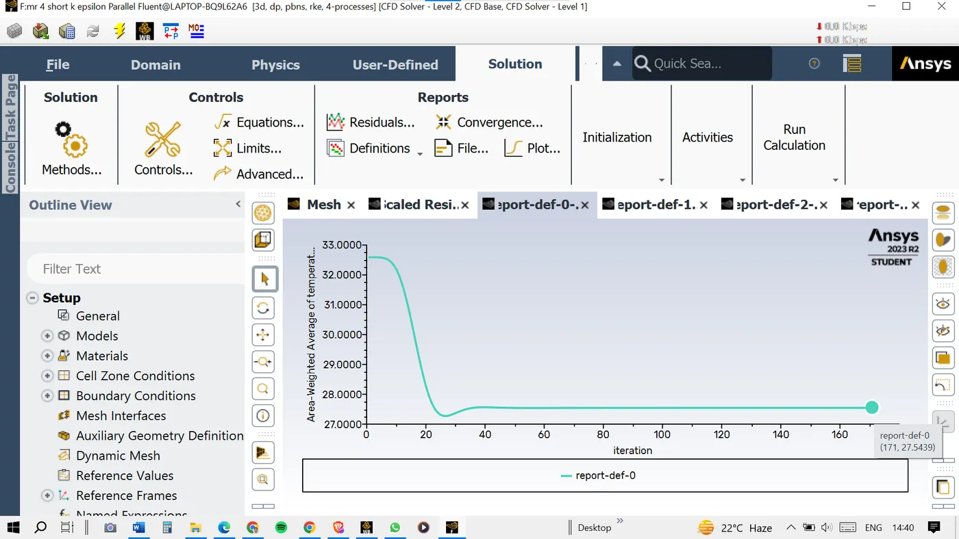
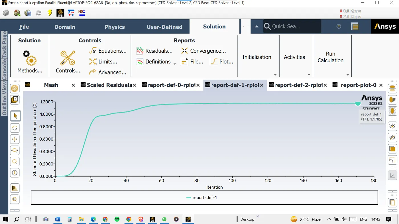
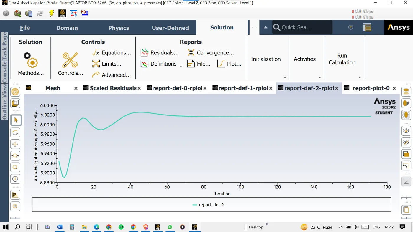
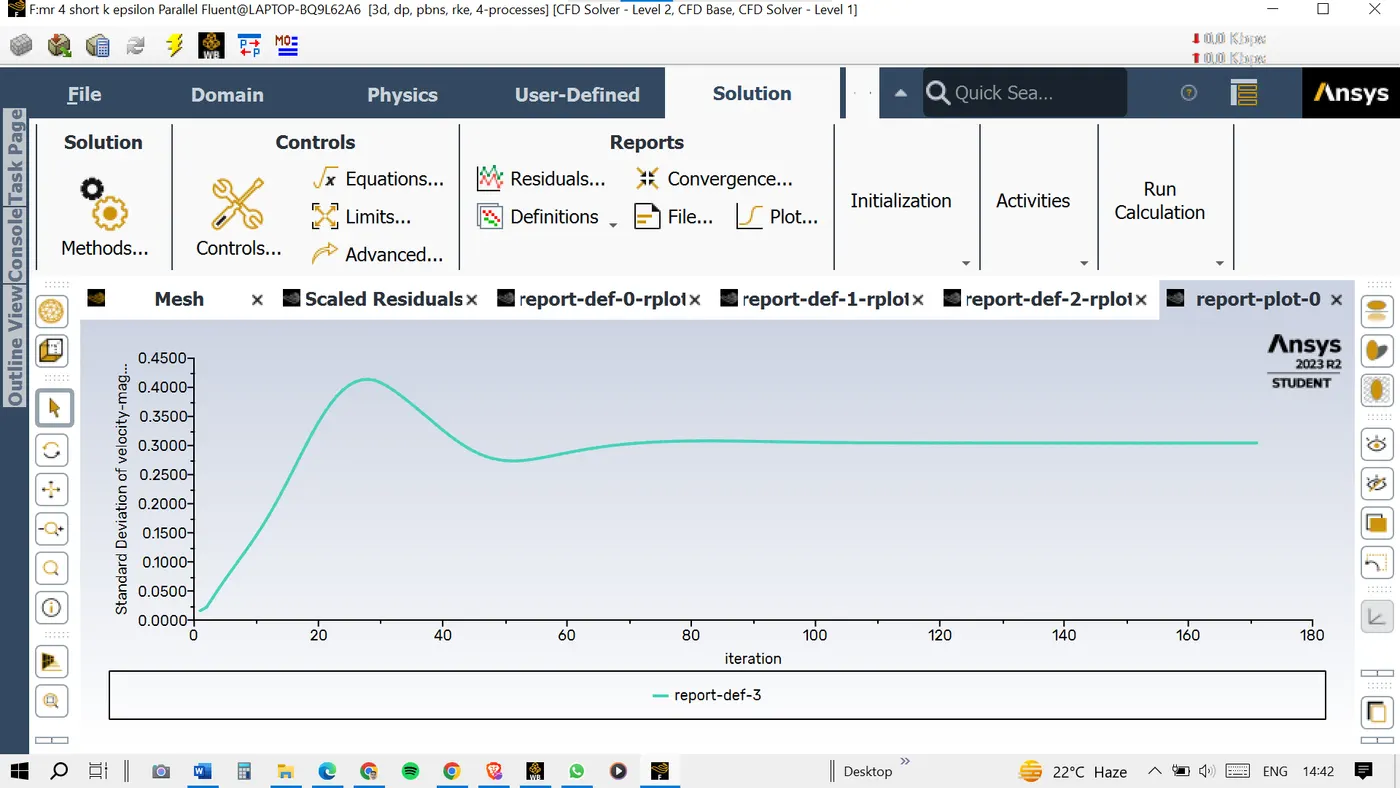
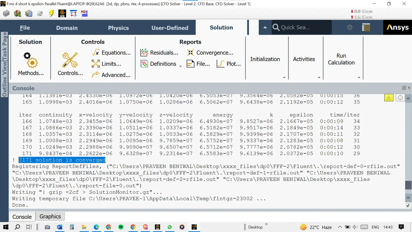
No. of iterations to converge = 171

Standard deviation = 1.1785

Area weighted average temperature = 27.5439

TEMPERATURE CONTOUR:

VELOCITY CONTOUR:

TEMPERATURE STREAMLINES:

VELOCITY STREAMLINES:

Case:2 Long Mixing Tee

Case2.1: Momentum Ratio=2

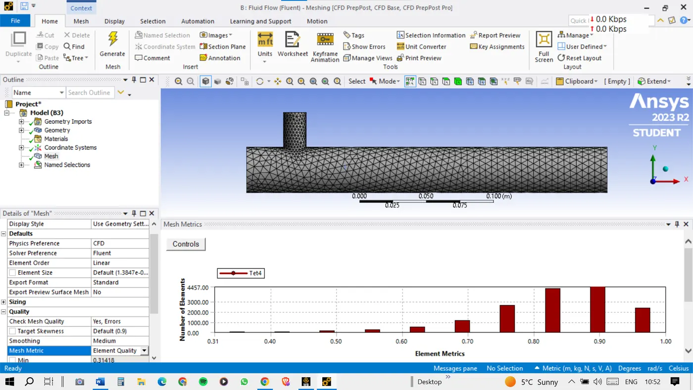
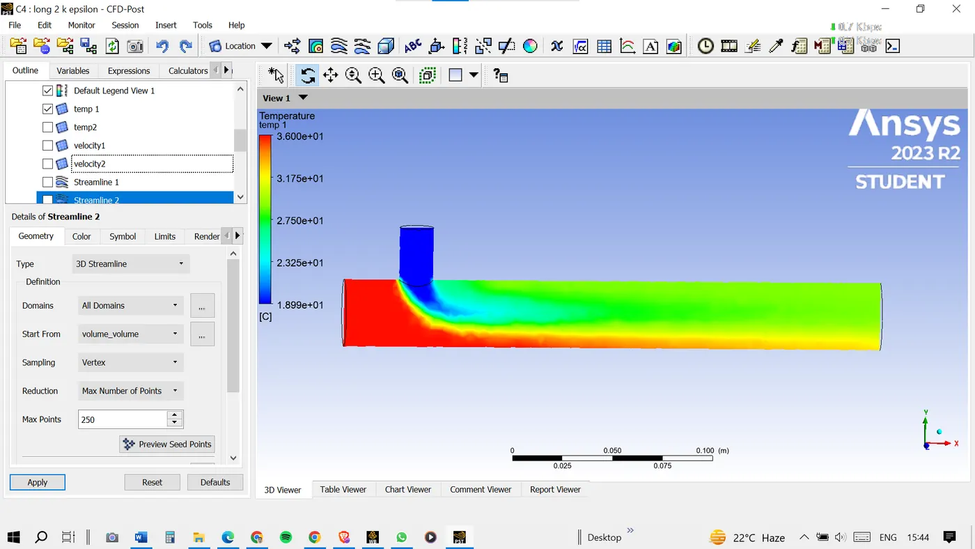
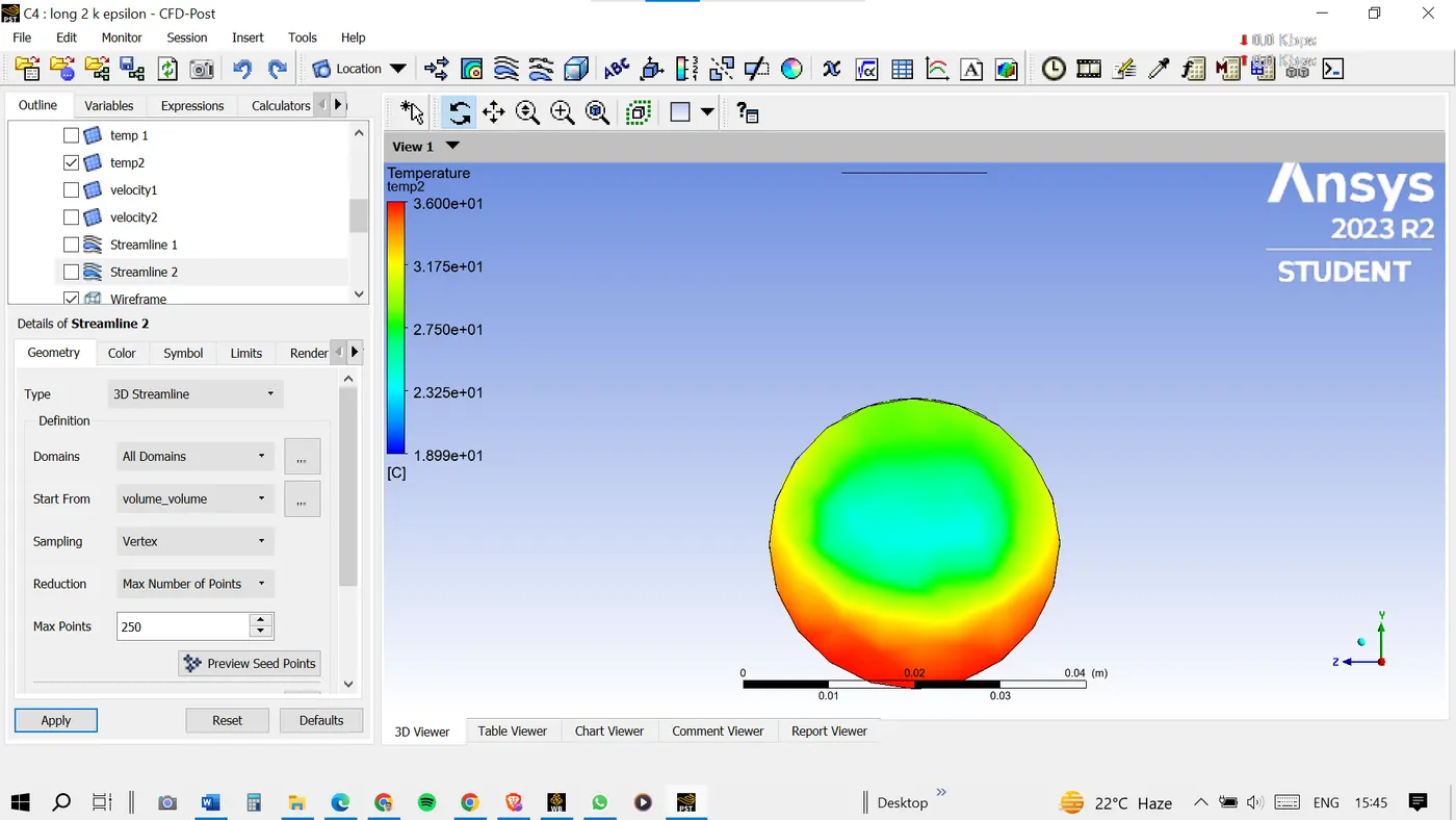
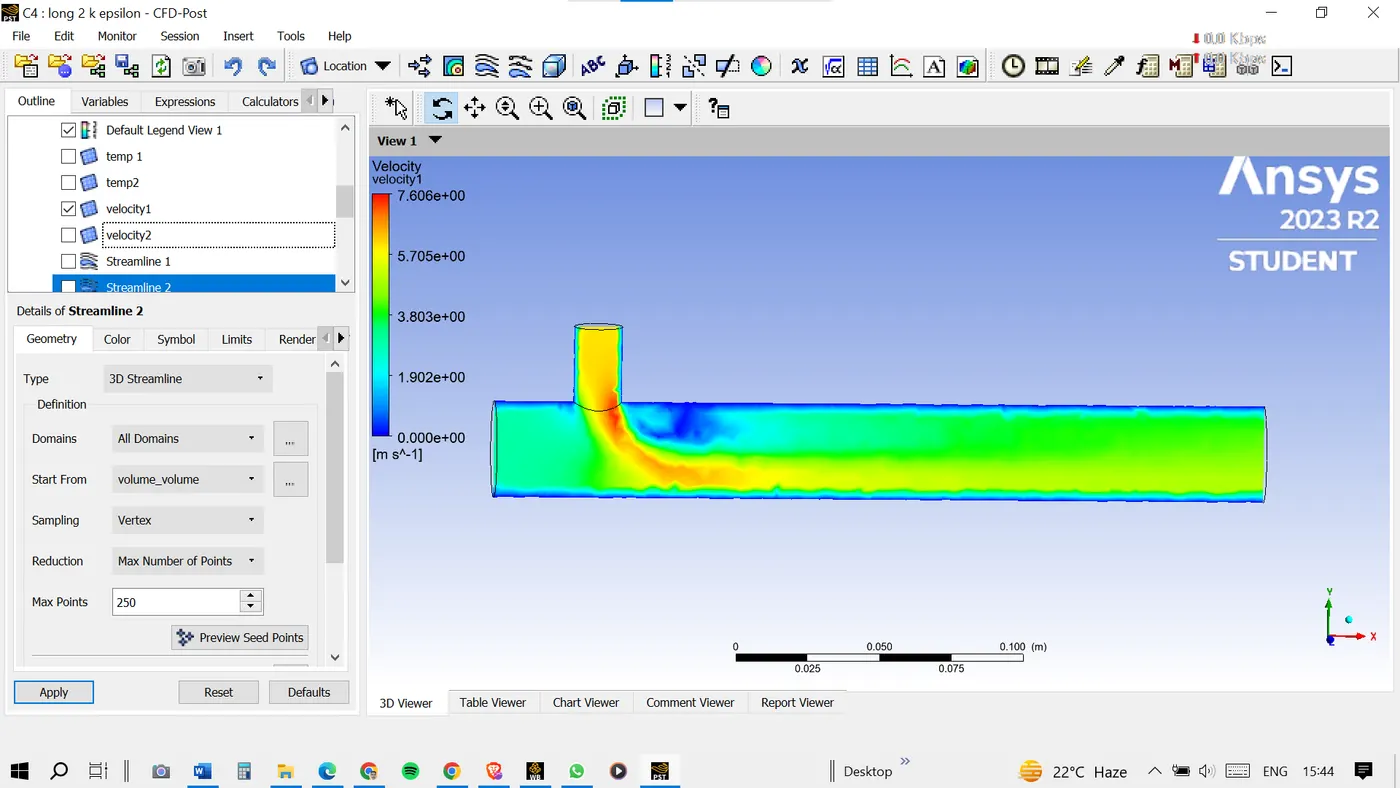
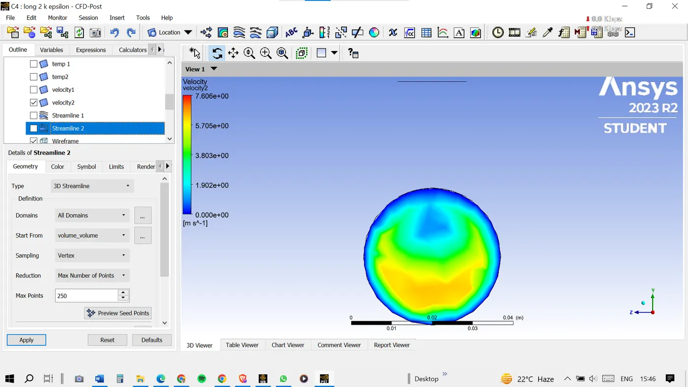
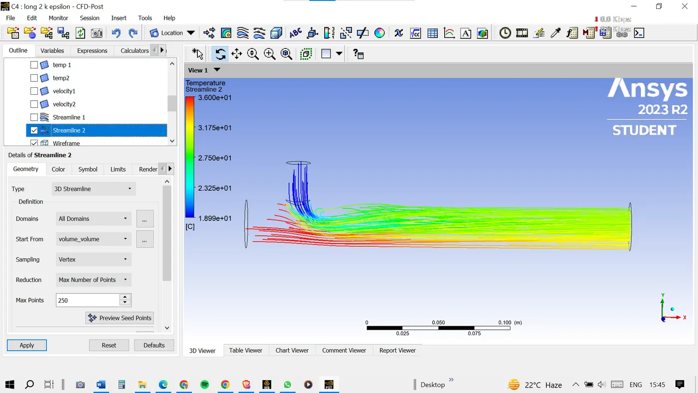
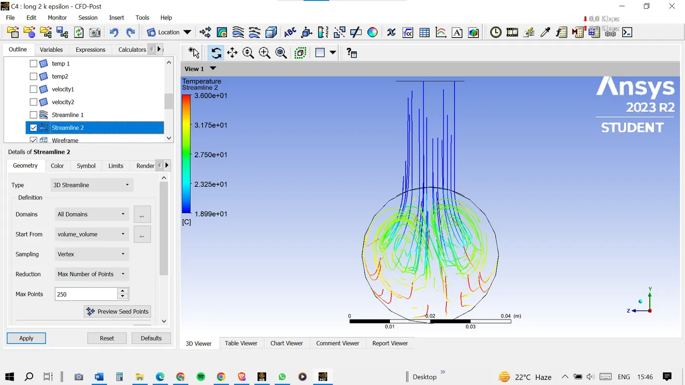
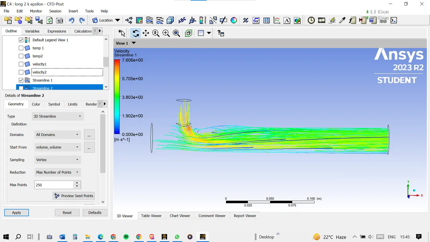
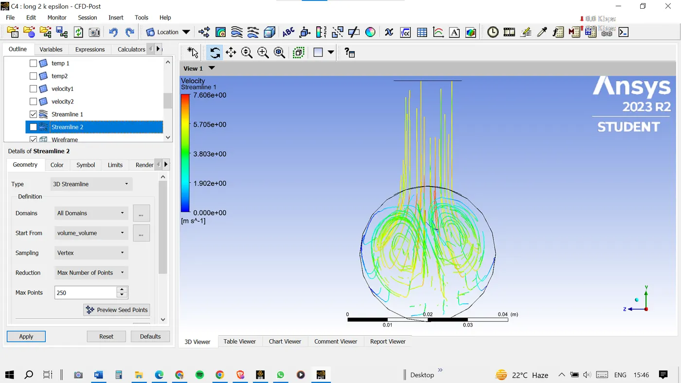
Plots for the long tee with MR=2 k epsilon

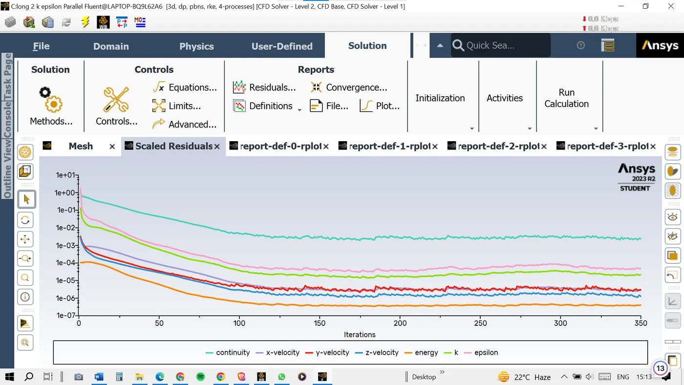
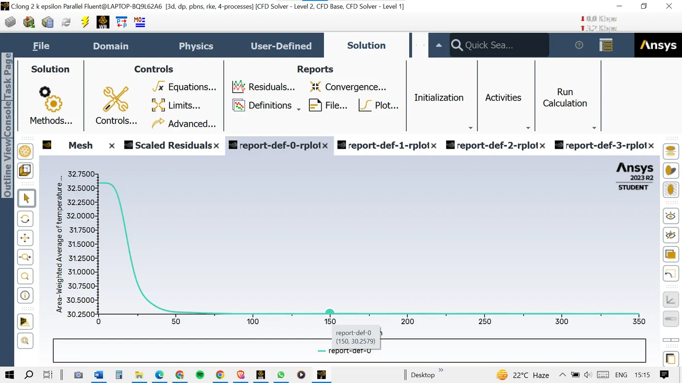
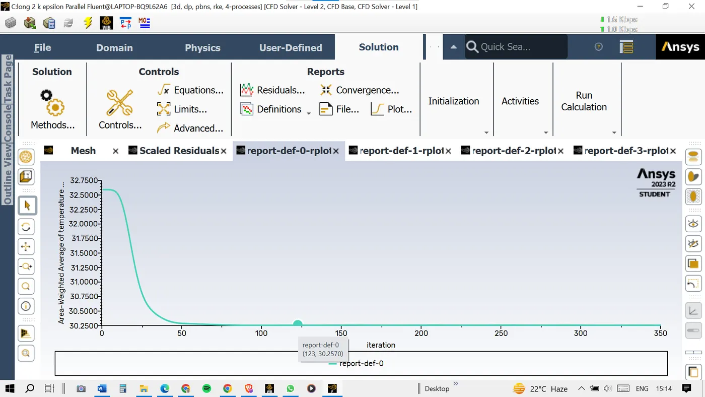
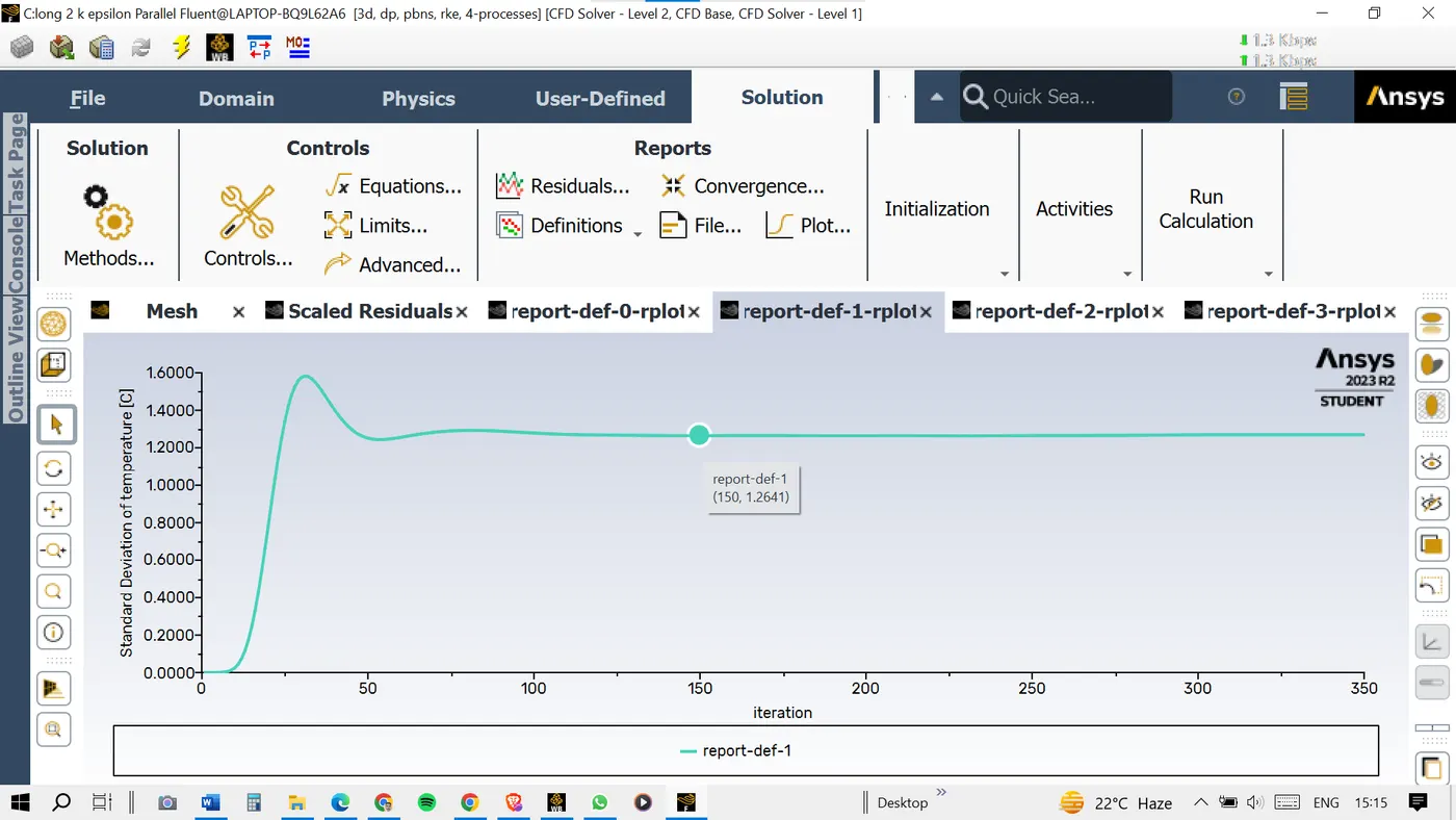
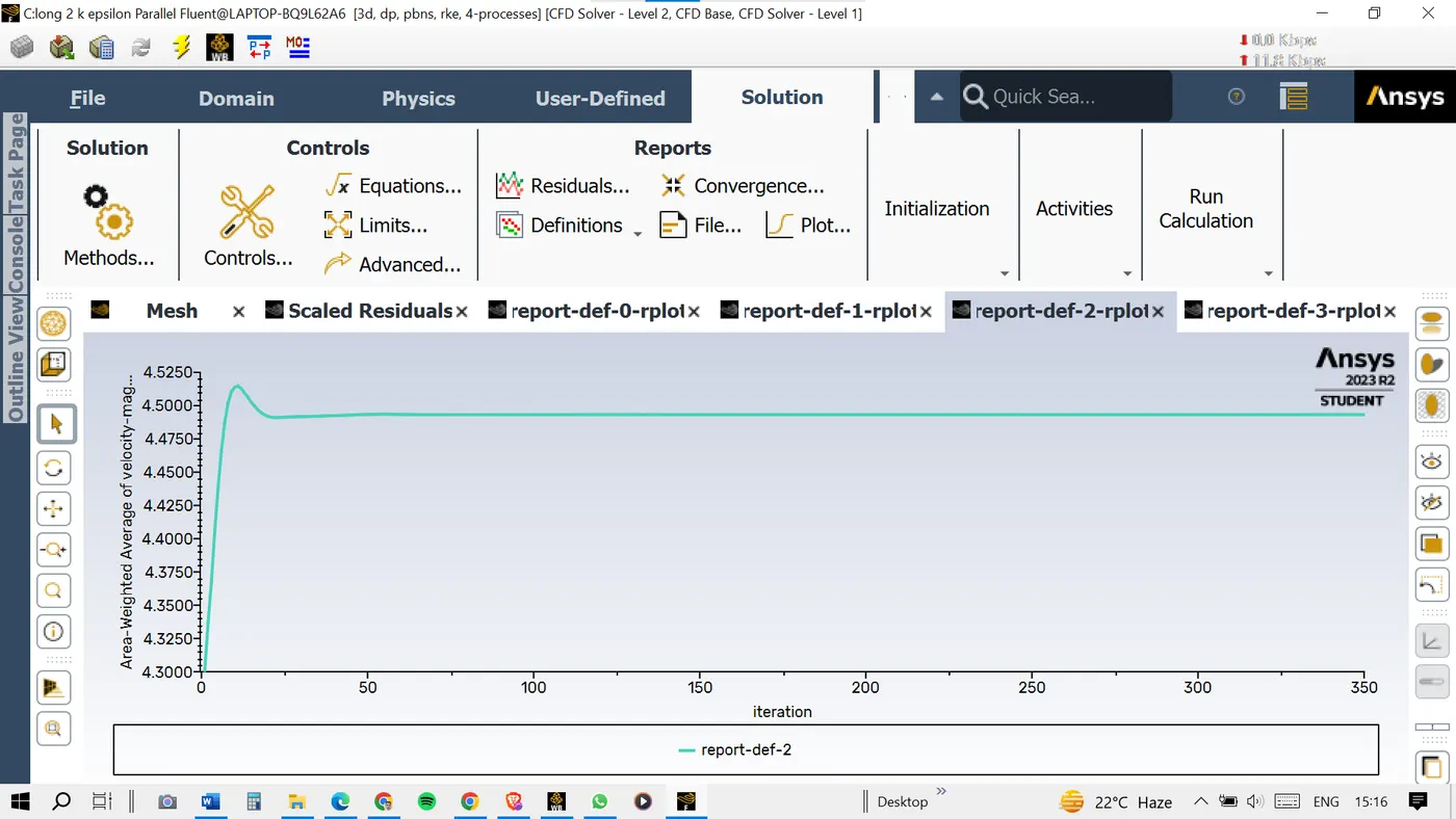
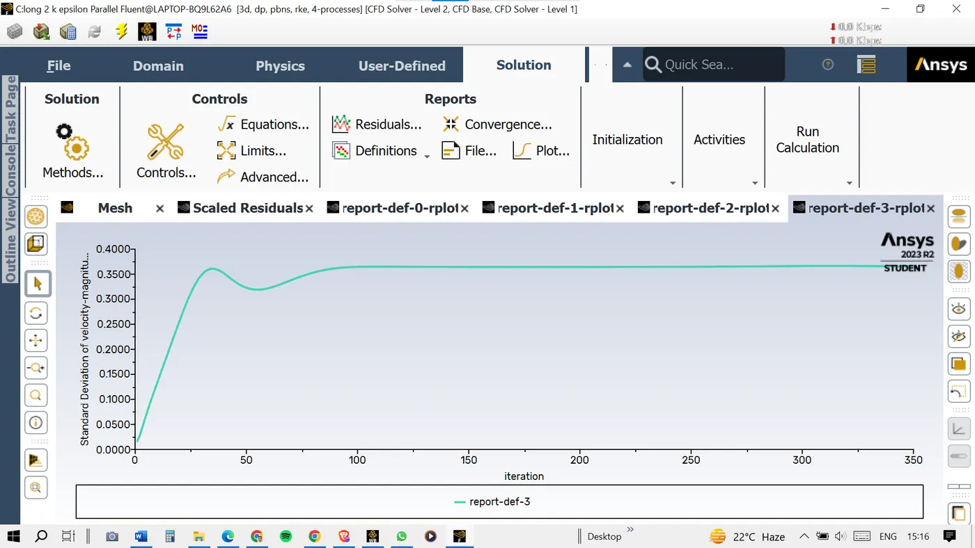
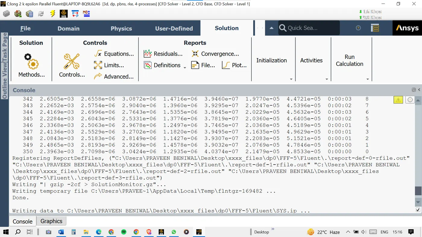
No. of iterations to converge = 120-150

Standard deviation = 1.264

Area weighted average temperature =30.257

TEMPERATURE CONTOUR:

VELOCITY CONTOUR:

TEMPERATURE STREAMLINES:

VELOCITY STREAMLINES:

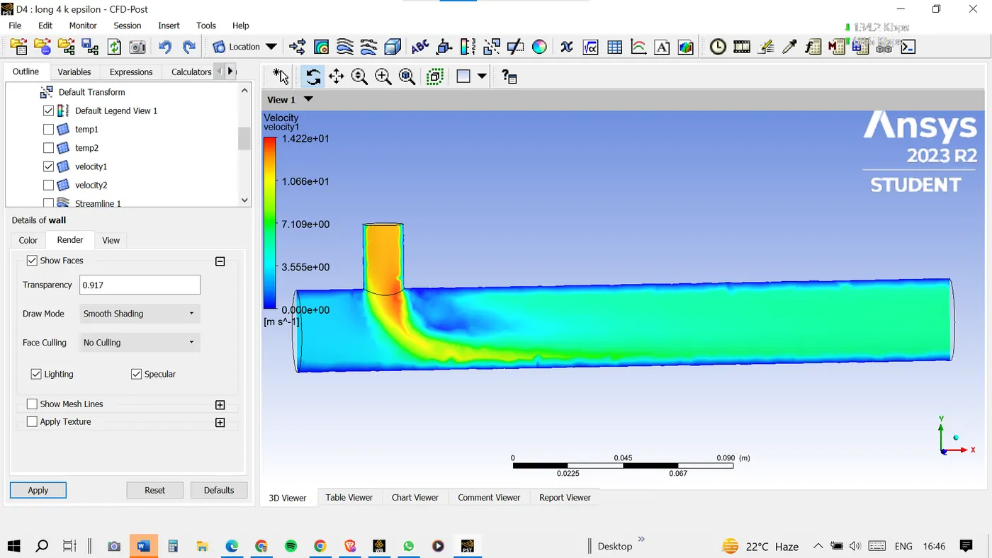
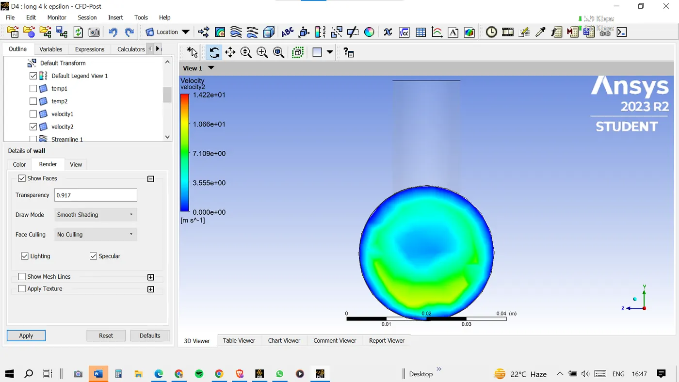
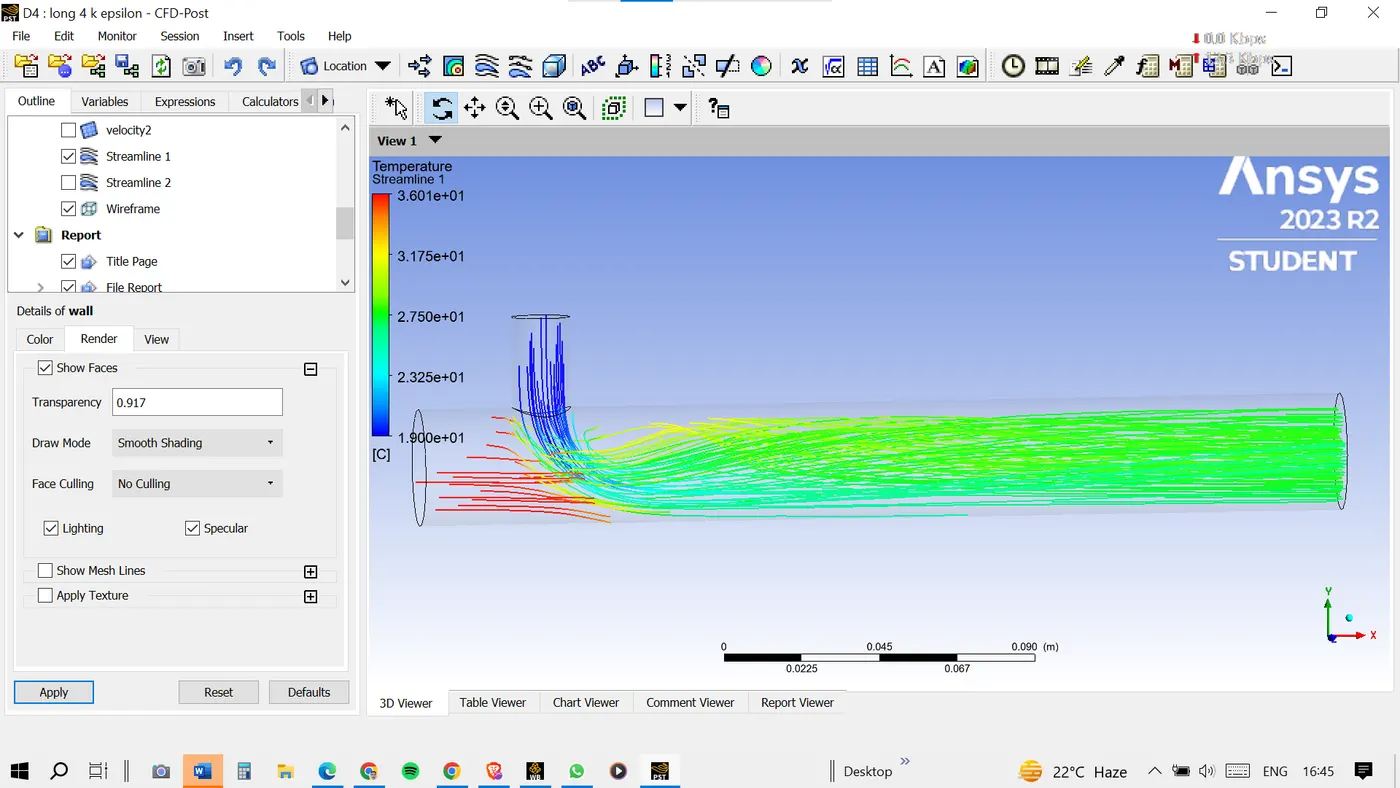
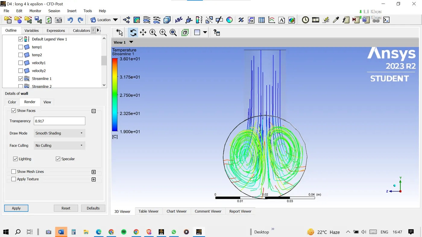
Case2.2: Momentum Ratio=4

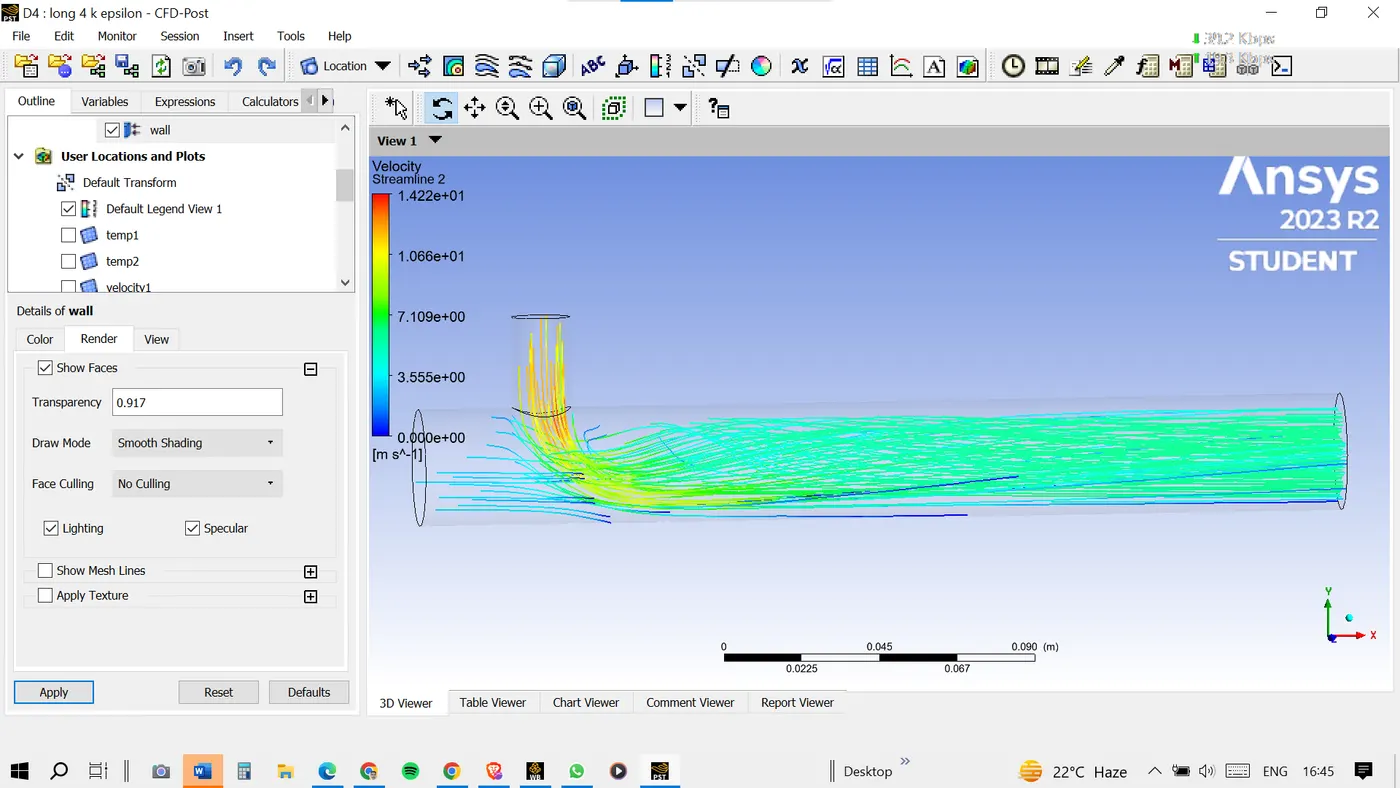
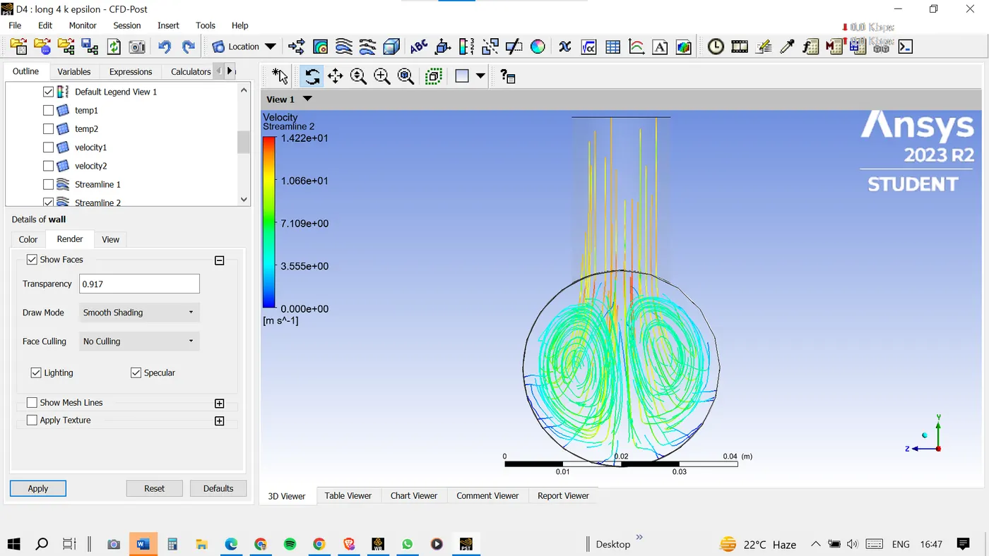
Plots for long tee MR=4 k-epsilon

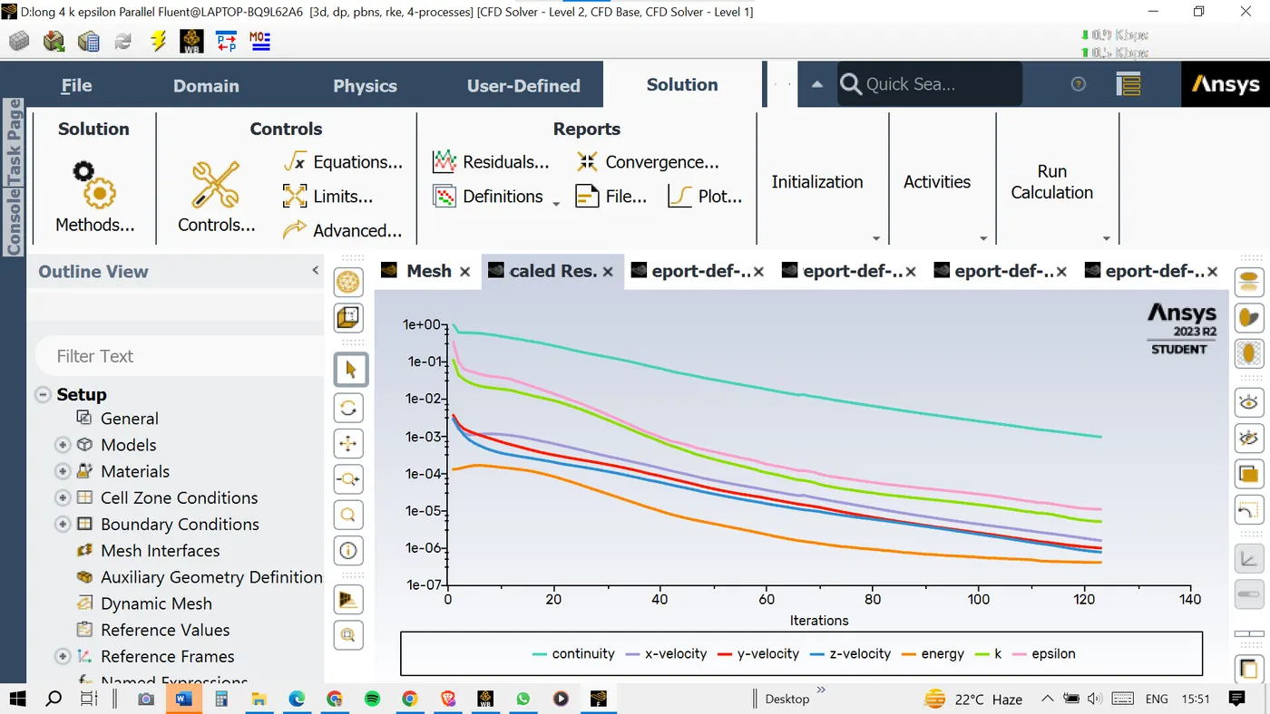
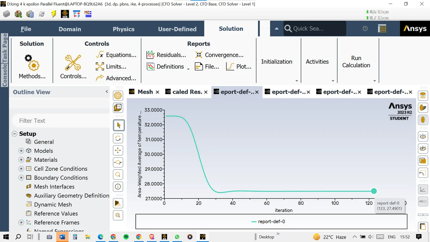
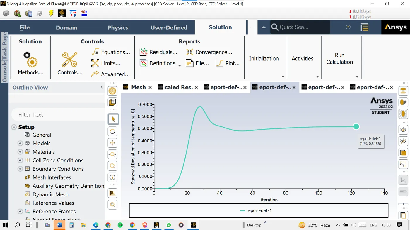
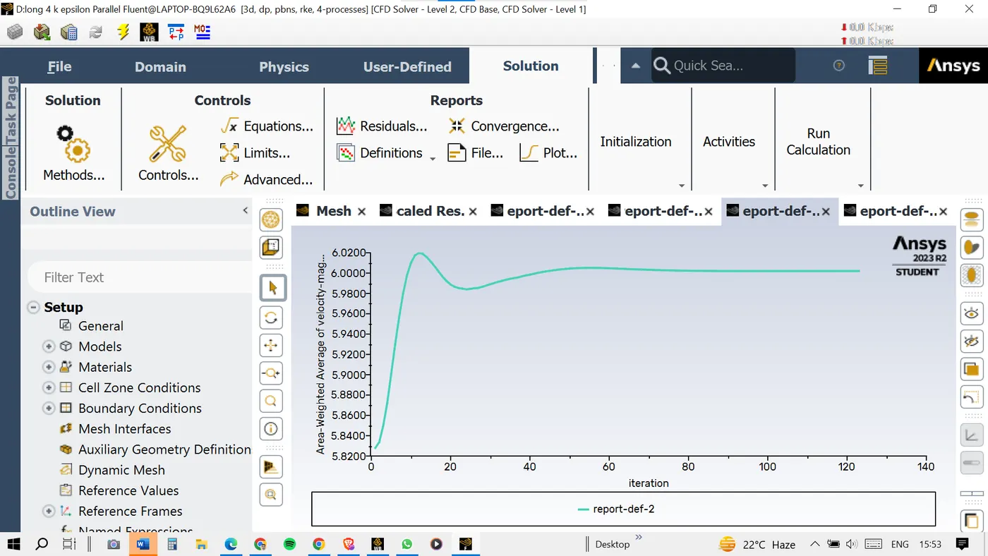
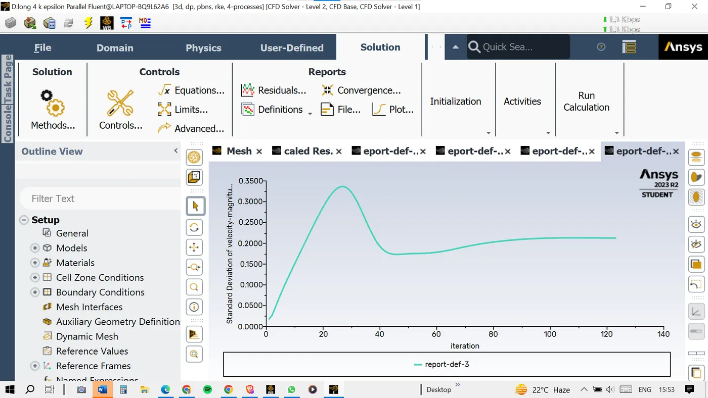
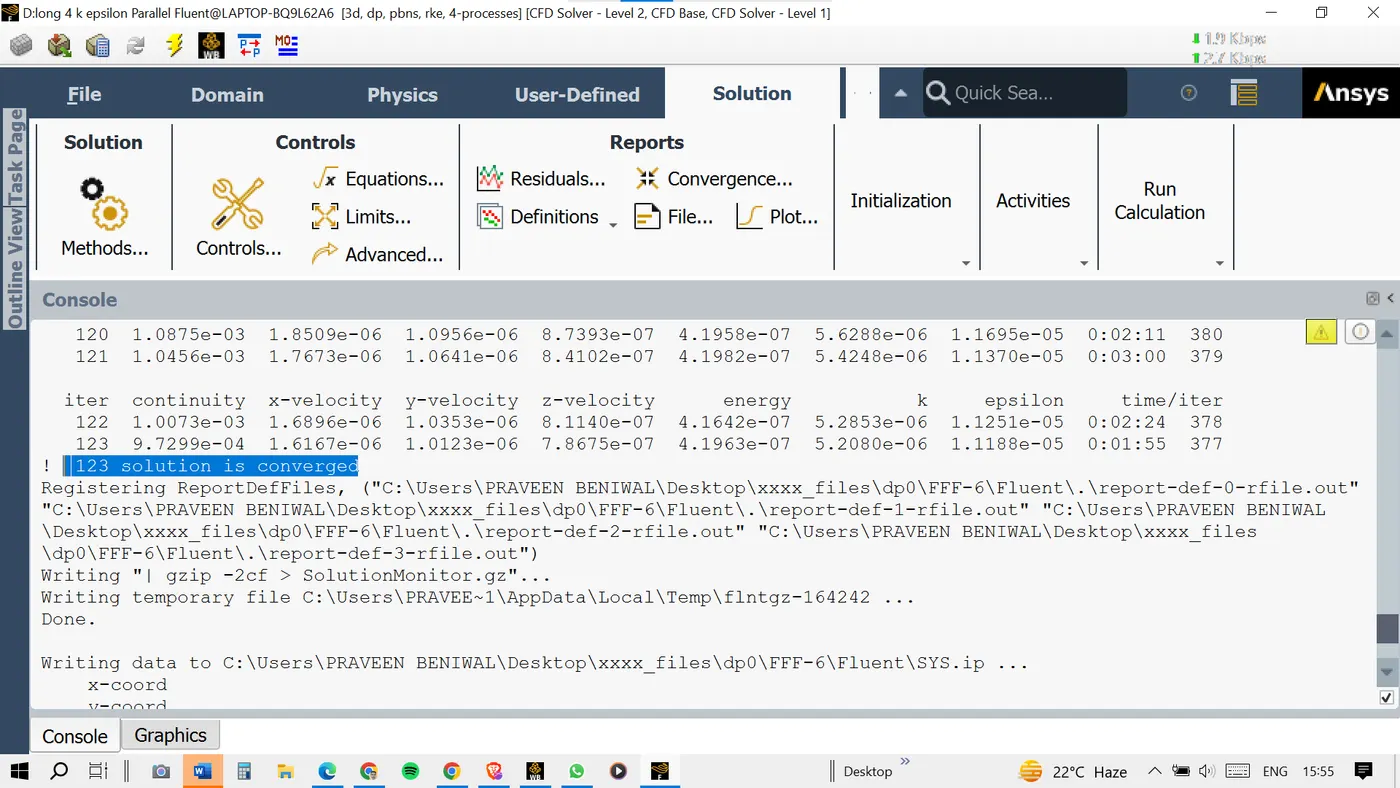
No. of iterations to converge = 123

Standard deviation = 0.5155

Area weighted average temperature = 27.4901

TEMPERATURE CONTOUR:

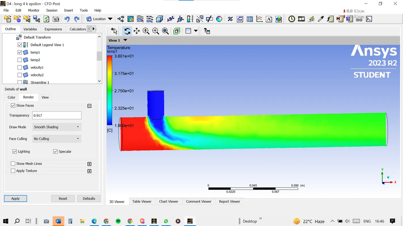
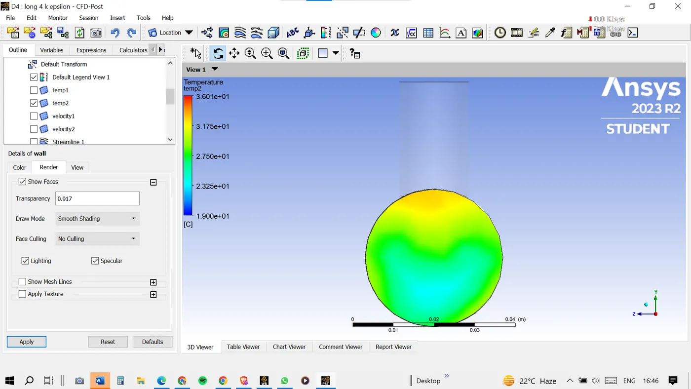
VELOCITY CONTOUR:

TEMPERATURE STREAMLINE:

VELOCITY STREAMLINES:

ANALYTICAL SOLUTION:

Formula,

TMixture = (mhot*Thot+mcold*Tcold )/(mhot+mcold)

Where,

Tmixture = average outlet temperature

mhot = mass flow rate of hot fluid = ᵨ .A.Vhot

mcold = mass flow rate of hot fluid = ᵨ .A.Vcold

Thot = temperature at hot inlet

Tcold = temperature at cold inlet

Calculations:

Case 1.1:

Thot= 360C, Tcold= 190C, Vhot= 3m/s, Vcold= 6m/s, Acold= 221.42 mm2, Ahot= 891.86 mm2, ᵨair = 1.225 kg/m

mhot = ᵨ .A.Vhot = 1.225*891.86*3 = 3277.58 kg/s

mcold = ᵨ .A.Vcold = 1.225*221.42*6 = 1627.43 kg/s

Tmixture =[(3277.58*36)+(1627.43*19)] / (3277.58+1627.43) = 30.3590C

Similarly,

Case 1.2: Tmixture = 27.5290C

Case 2.1: Tmixture = 30.3760C

Case 2.2: Tmixture = 27.5490C

FINAL RESULTS :

The table below shows the obtained data in the two cases and also the comparison with the analytical solution.

TABLE

Mixing Tee Length		SHORT		LONG
Momentum Ratio		2	4	2	4
Cell count		12692	12692	15727	15727
Average outlet temperature(C)	Numerical	30.263	27.543	30.257	27.490
	Analytical	30.359	27.529	30.376	27.549
Number of iterations for convergence		155	171	120-150	123

KEY OBSERVATIONS FROM THE RESULT:

· Higher momentum ratios contribute to lower outlet temperatures, suggesting enhanced mixing.

· Longer mixing tees generally exhibit lower average outlet temperatures, indicating improved mixing efficiency, but not with a great difference.

MESH INDEPENDENCE TEST

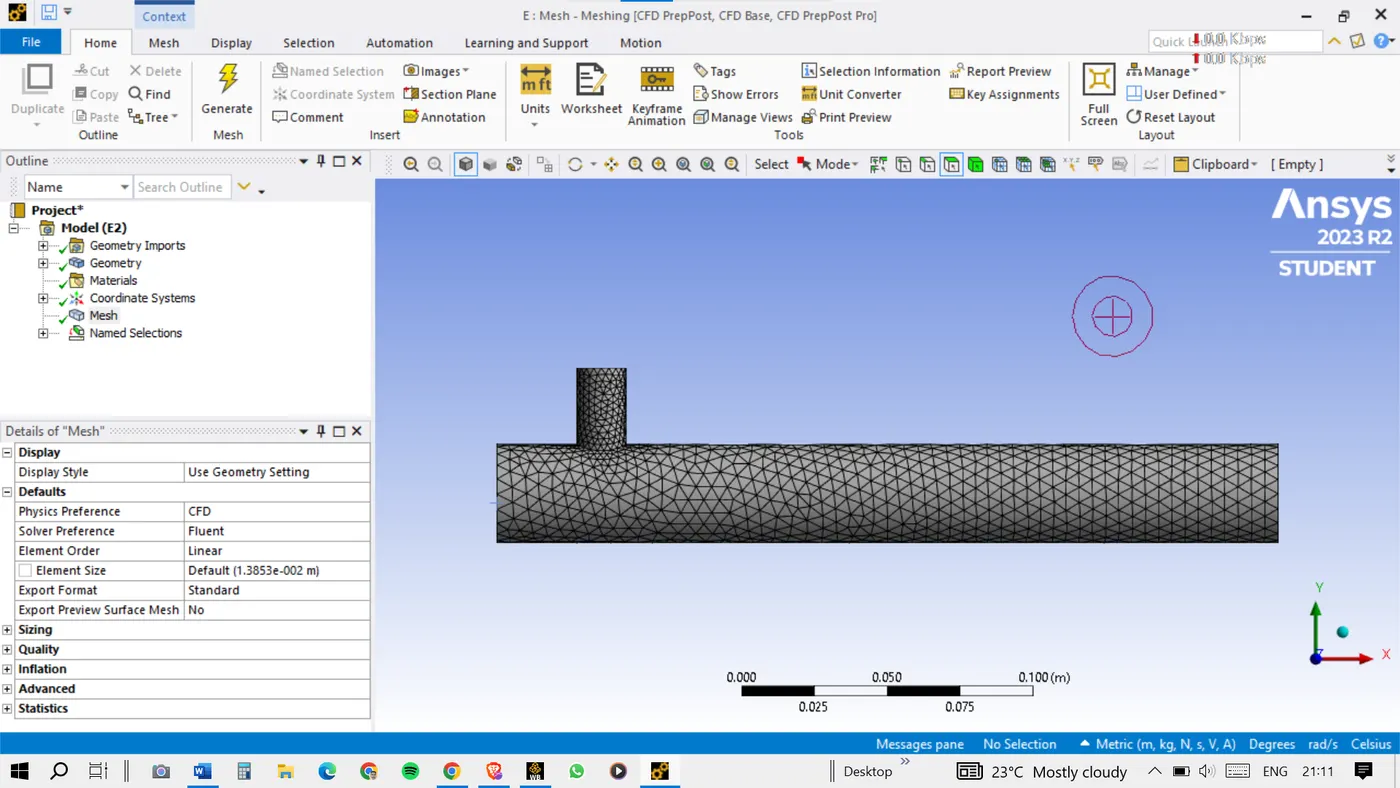
Here we will test the impact of mesh size on the results of the simulation. We will simulate with three different sizes and note down the result to determine the impact on the final output of the simulation.

Mesh sizes are:

· Default

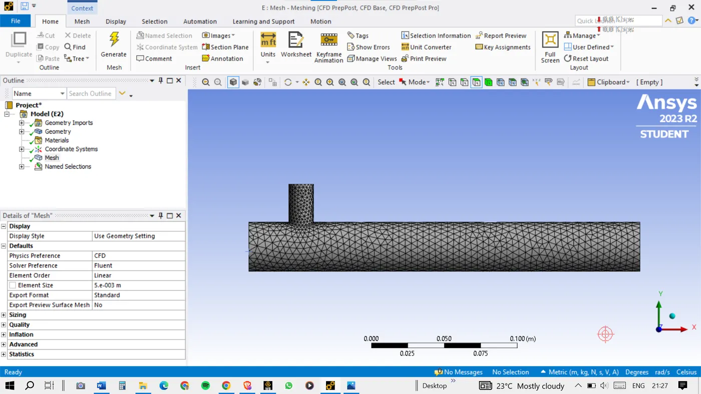
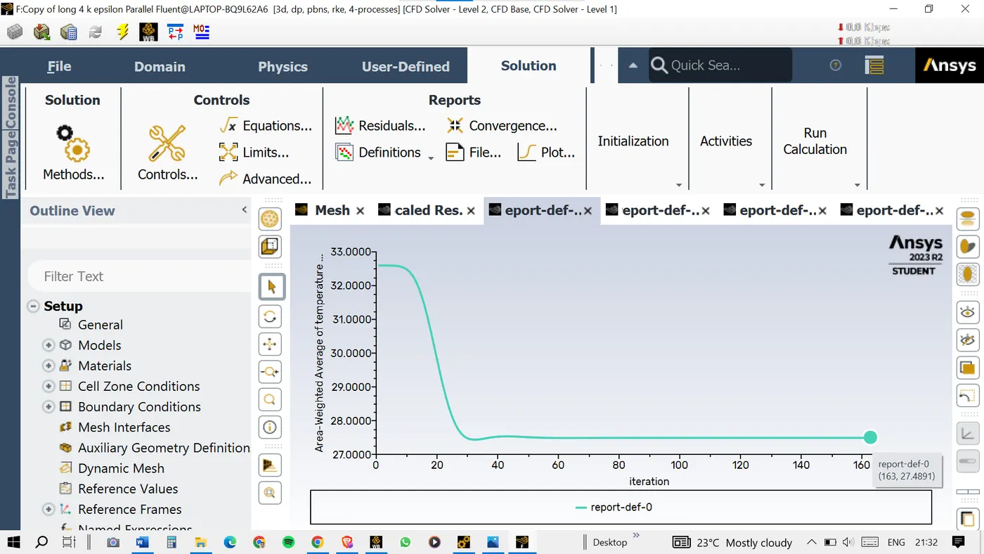
· 0.005

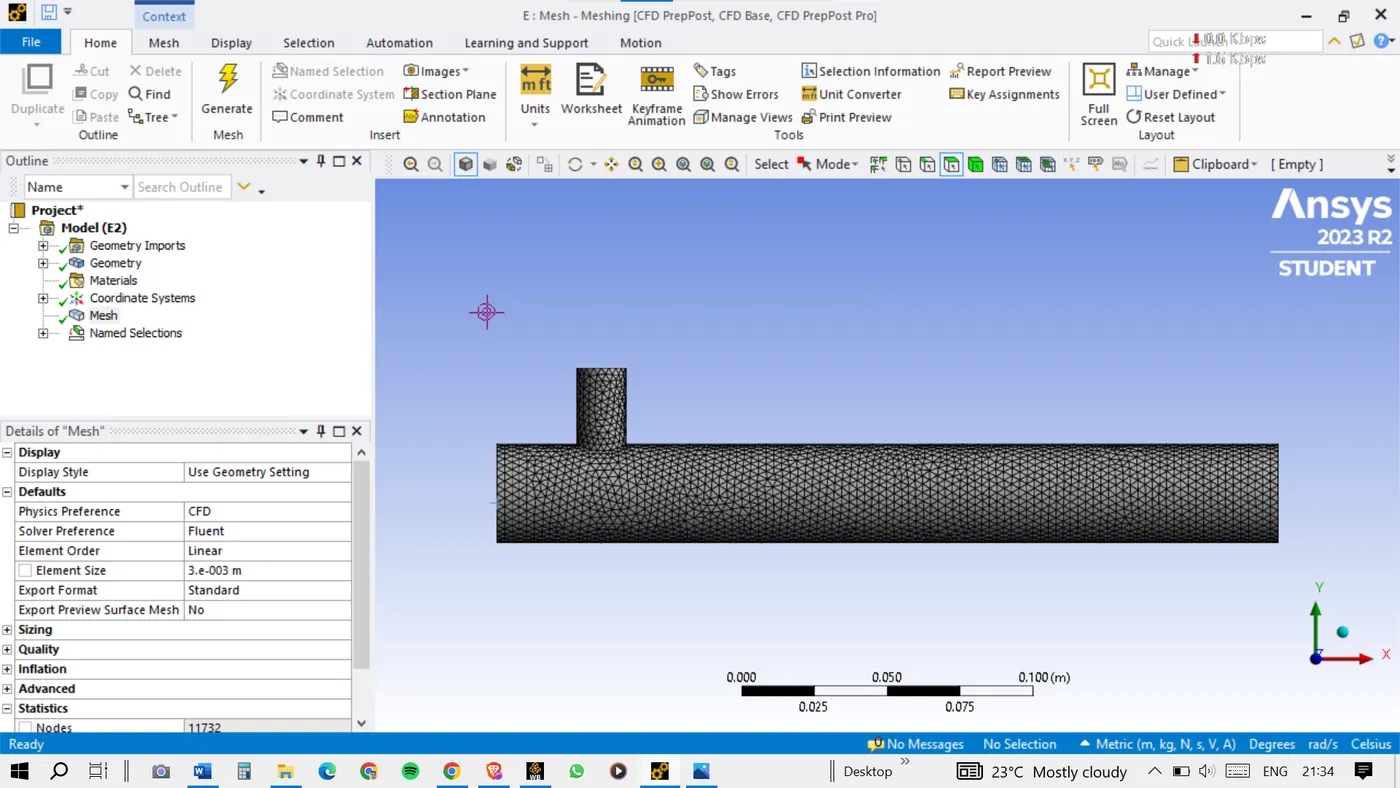
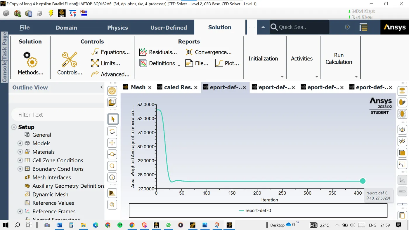
· 0.003

DEFAULT ELEMENT SIZE:

ELEMENT SIZE 0.005:

ELEMENT SIZE 0.003:

RESULT :

This table shows the impact of mesh size on the final output of the simulation.

MESH INDEPENDENCE TEST
Element size	Default	0.005	0.003
Cell count	15727	18069	56670
Average outlet temperature(C)	27.490	27.4891	27.5323
Standard deviation	0.5155	0.5683	0.5704

KEY OBSERVATIONS FROM THE ABOVE RESULT:

· The average outlet temperature remains consistent across different mesh sizes, with variations within an acceptable range.

· Standard deviation values are comparable, indicating stability in the simulation results.

· The results suggest that the simulation is relatively independent of mesh size.

· The default mesh with 15727 cells provides reliable results, and finer meshes do not significantly alter the outcomes.

CONCLUSION:

Turbulence Model Choice:

· Realizable k-ε turbulence model selected for further cases due to lower standard deviation, indicating more efficient mixing compared to the k–ω model.

Momentum Ratio Influence:

· Higher momentum ratio and increased cold air inlet velocity result in more efficient cooling.

· Increasing the cold inlet velocity enhances cooling efficiency.

Tee Length Impact:

· Longer tee geometry leads to lower standard deviation, indicating improved fluid mixing.

· Tee length doesn't significantly affect outlet temperature compared to a short mixing tee.

Mesh Independence Test:

· Negligible change in average outlet temperature and standard deviation among different mesh sizes.

· Simulation deemed mesh-independent, with increased mesh size providing more accurate results.

Overall Conclusion:

· An increase in Cold inlet velocity enhances cooling efficiency.

· Tee length extension improves fluid mixing.

· The realizable k-ε model offers reliable predictions for efficient simulations.