Mixing Tee Challenge

Problem Statement:

Solve the mixing of hot and cold fluid diffusion for a given problem using work bench and fluent under steady-state simulations and compare the mixing effectiveness when hot inlet temperature is 36°C & the Cold inlet is at 19°C. Use the k-omega SST model for all cases.

Case 1: Short mixing tee with a hot inlet velocity of 3 m/s and Momentum ratio of 2 & 4.

Case 2: Long mixing tee with a hot inlet velocity of 3 m/s and Momentum ratio of 2 & 4.

In a table, compare the following values from the 2 cases.

• Cell count
• Average outlet temperature (Theoretical & Numerical)
• Number of iterations for convergence

Aim :

• For this challenge, we have created two versions of the mixing tee. One of them is longer than the other.our job is to set up steady-state simulations to compare the mixing effectiveness when hot inlet temperature is 36⁰C & the Cold inlet is at 19⁰C Use the k-epsilon and k-omega-SST model for the first case and based on your judgment use the more suitable model for further cases. Giving the reason for choosing a suitable model is compulsory.

Objectives :

1. Velocity and temperature contour plots on the cut planes along and across the pipe.
2. Velocity and temperature line plots along and across the length of the pipe.
3. Perform Mesh independent study for any one case.
4. Discuss the effect of length and momentum ratio on results.

For each simulation, I need to show the convergence plot .

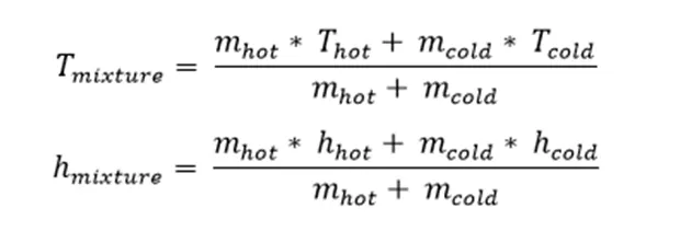
Reference ormulas:-

Theory :

1. Introduction to fluid :

• Fluid is a substance i.e. having the ability to flow or deform(angular) continuously under the action of shear force(no matter how much small the force).
• Generally liquids and gases falls in this category of fluids.
• Ex : water, air, petrol, steam, mercury etc.
• There are 3 ways we are studied on fluids
  1. Fluid statics – study of fluid at rest
  2. Fluid kinematics – study of fluid in motion without considering pressure forces
  3. Fluid dynamics – study of fluid in motion(i.e. with considering forces)

2. Fundamentals of fluid mechanics :

• Newton’s law of viscosity (NLV):
  • A fluid shear stress is defined as the tangential deformation of a fluid element when a force is applied to it.
  • The law states that , this shear stress is directly proportional to the normal velocity gradient experienced by that fluid element.
  • Mathematically it is given as

τ=μ(dudy)">τ=μ(du/dy)

Where

τ=shear stress (Pa or N/m²)

μ">μ= dynamic viscosity or viscosity(N-S/m² or Pa-S)

dudy">du/dy= velocity gradient (S^-1)

3. Types of fluids :

• Ideal fluid – it is a fluid which shows non-viscous, incompressible and zero surface tension in nature.
• Real fluid – possesses viscosity
• Newtonian fluid - which obeys NLV(Ex: oil,water,air etc.)
• Non-newtonian fluid – which does not obey NLV (Ex : blood,paints etc.)
• Ideal plastic fluid – in which shear stress is more than the yield value and obeys NLV.( Ex: toothpaste ,gels etc)
• Compressible fluid – a fluid in which the density of a fluid changes with change in the pressure or volume called as compressible fluids.(Ex : air)
• Incompressible fluid - a fluid in which the density of a fluid doesnot change w.r.t. change in pressure and volume.(Ex : water)

4. Introduction to mixing tee :

• Mixing tee is nothing but the there is a mixing of fluids in a T-joint.
• In this there are 2 inlets and 1 outlet. The 2 fluids with different properties are mixed in this joint and flows to the outside as a 1 fluid.
• The application of this model is in central air conditioning .

Procedure :

1. Case-1: Short mixing tee with Momentum ratio=2 :

• Open the workbench

• Now drag the fluid flow(fluent) to the workspace

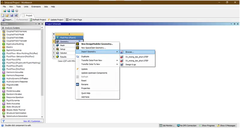
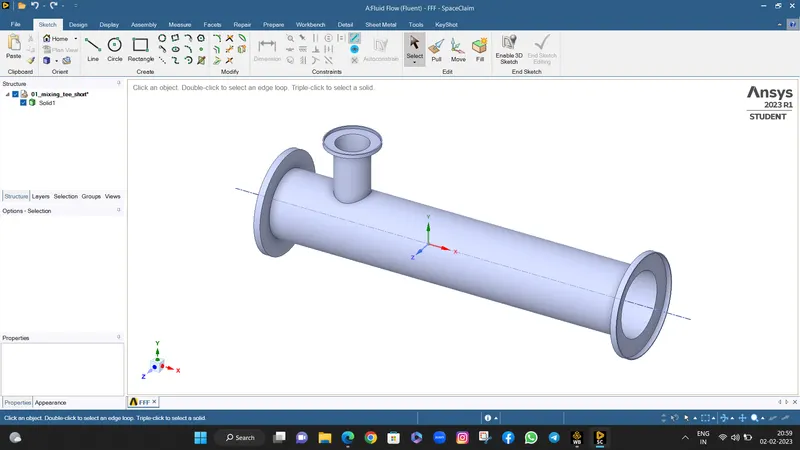
• Now right click on the geometry and import the short tee model

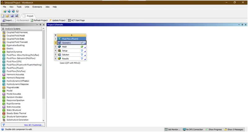
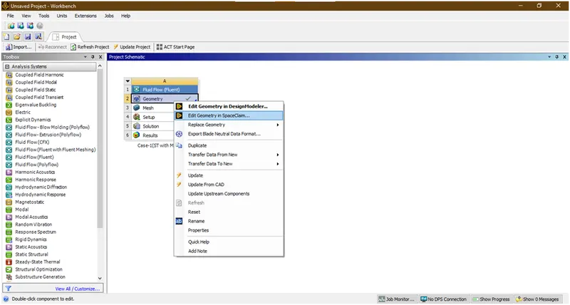
Now it has been imported.Now right click on geometry and click on edit with spaceclaim

Now goto prepare and extract the volume

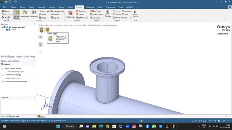
Now select the edges

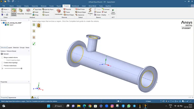
Now click on green tick and here the volume has been extract.

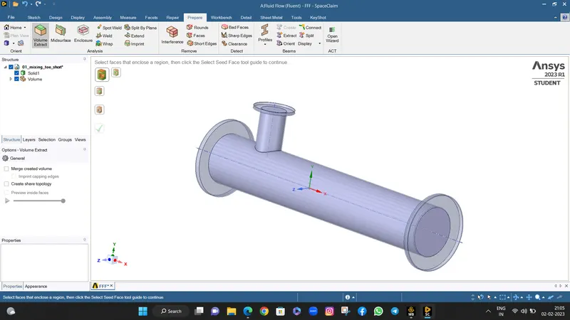
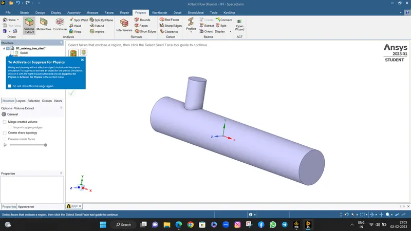
Now suppress the solid part for further physics. for that right click on shell and then click on ‘supress for physics’

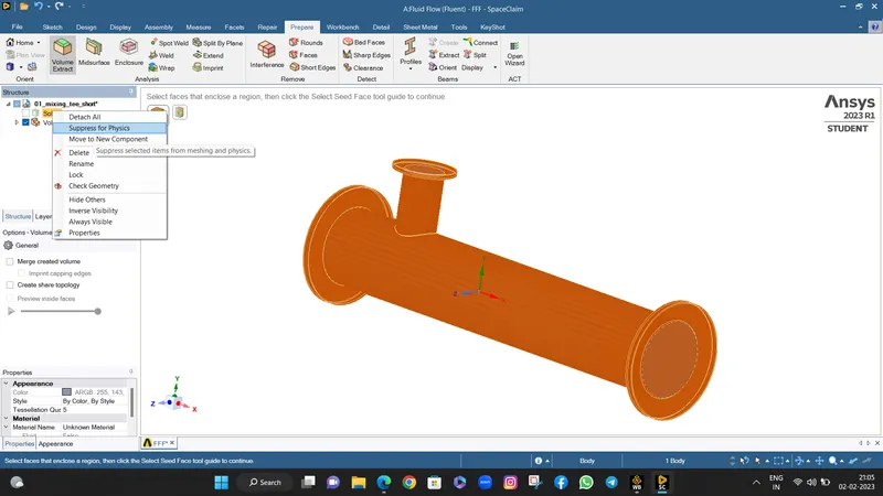
Now it has been suppress and shows symbol as not as highlited.now close this spaceclaim.

• Now right click on mesh and goto edit and wait for open

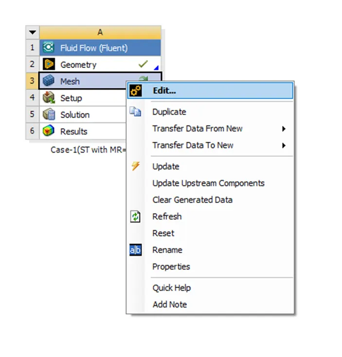
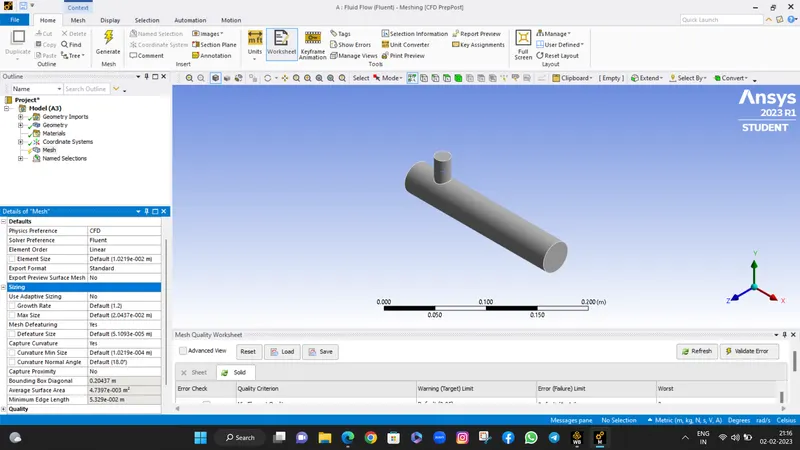
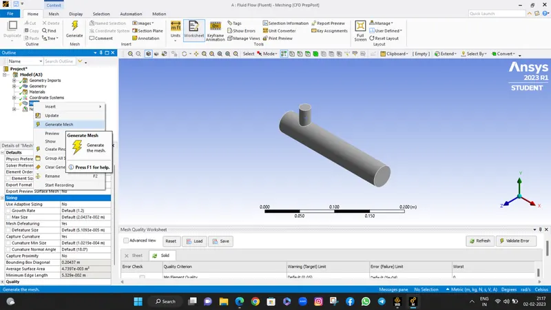
This is showing by default mesh element size .

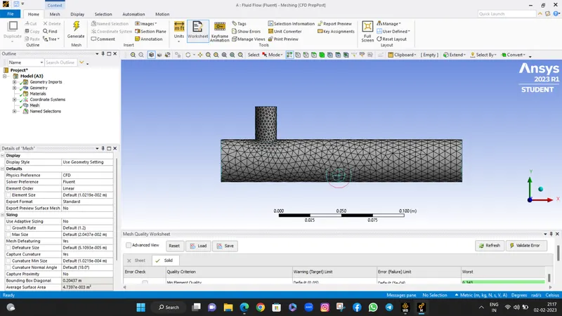
Now change the element size=2mm

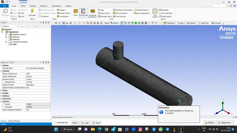
Let select the faces and gives names to the faces.

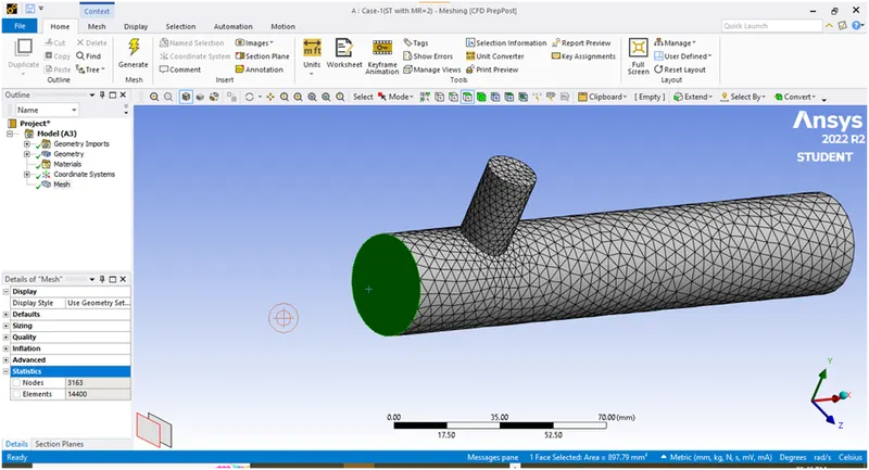
Now give name as ’Inlet-x’.to give this press short-cut key ‘N’ or right click on face and goto create name selection

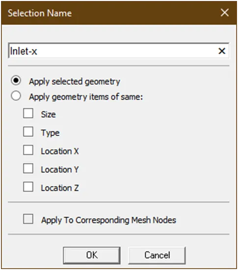
Now type the name and click on ok.

Similarly we are giving the names as ‘Inlet-y and outlet’

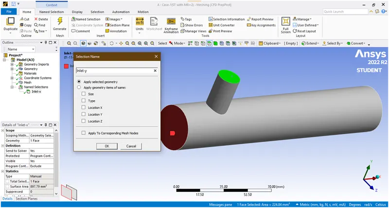
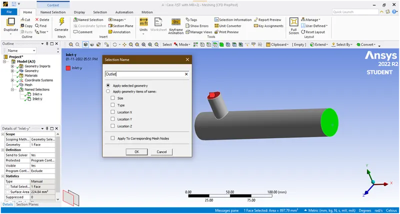
Now right click on mesh->update to update this data to fluent

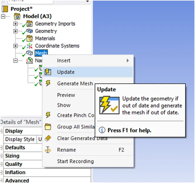
After that close this mesh window.

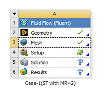
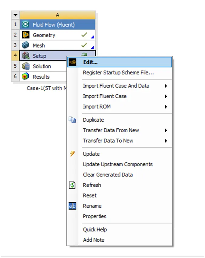
• Now right click on setup->edit

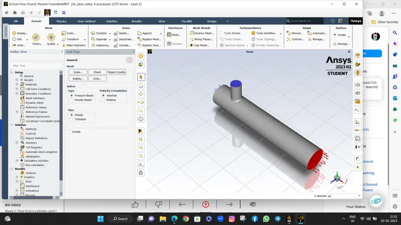
A new popup opens, Now click on double precision and solver processes=4 then click on start and wait to open ansys fluent.

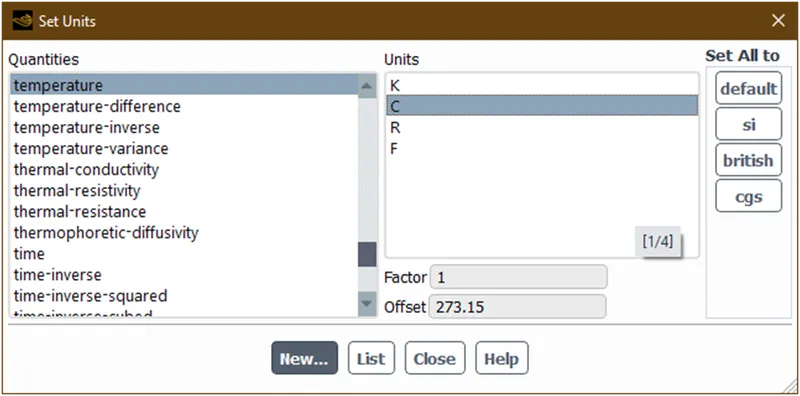
Now goto units and find temperature and set unit as celcius

Now double click on energy and enable.this model is used for thermal energy calculations

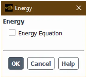
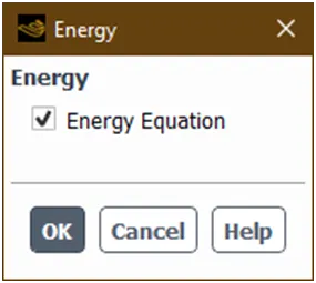
Now double click on viscous model

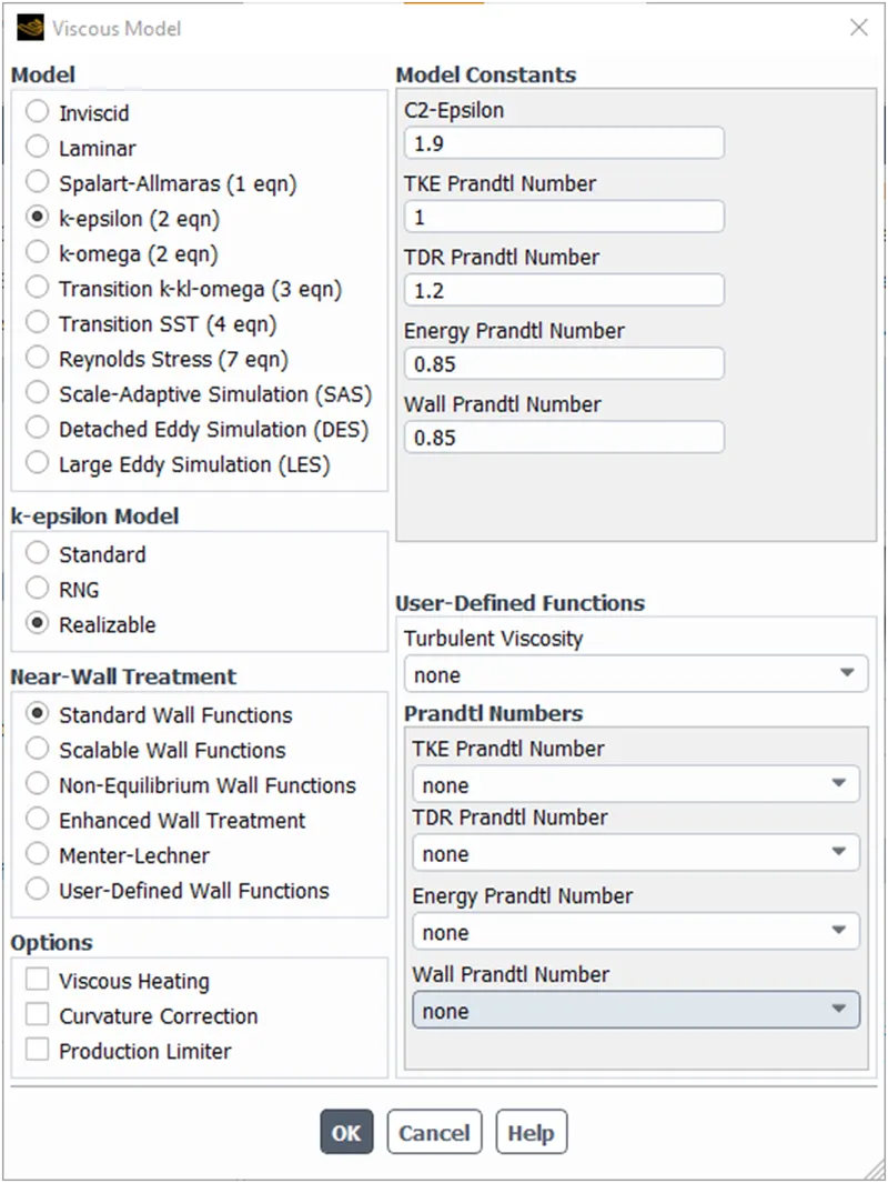
Now select k-epsilon->realizable->standard wall function->click on ok.

Here we are doing analysis by using air.so no need to change.it has been default selected.

Now goto cell zone and apply material.

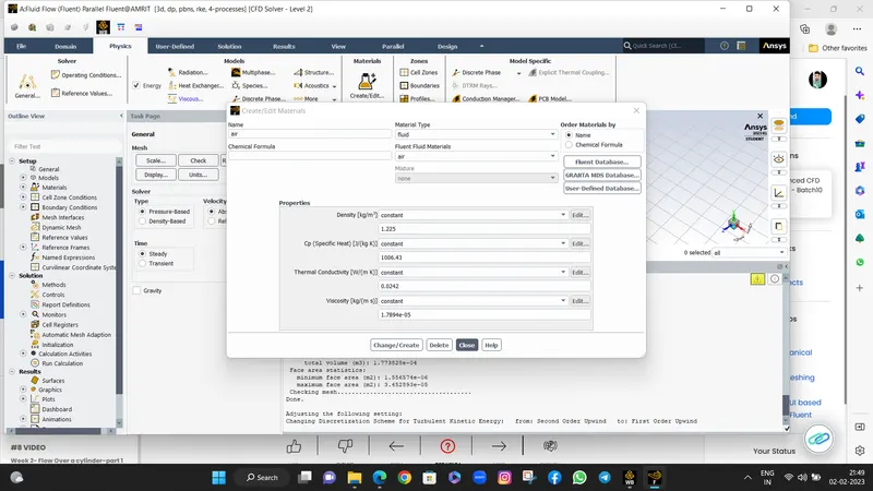
Default air has been selected click on apply and close this tab.

Lets goto the boundary

Now click on inlet-x

Select the velocity specification method as shown above and here the velocity magnitude is given as 3m/s so give the value and goto the thermal section

Now from inlet-x the hot fluid enter so here the temp given as=36 C so put this value and apply and then close

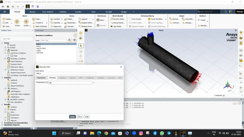
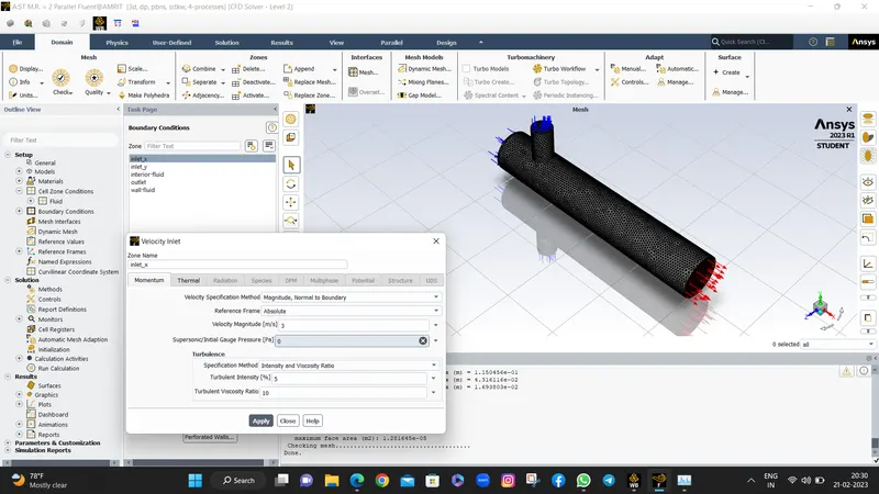
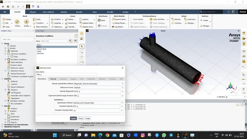
Now double click on inlet-y.here this also a velocity inlet type.

Now give velocity value.here velocity is given in terms of momentum ratio=2

Momentum ratio = velocity at cold inlet / velocity at hot inlet

From above formula by keeping the values we are getting

velocity at cold inlet=momentum ratio * velocity at hot inlet = 2 * 3=6 m/s

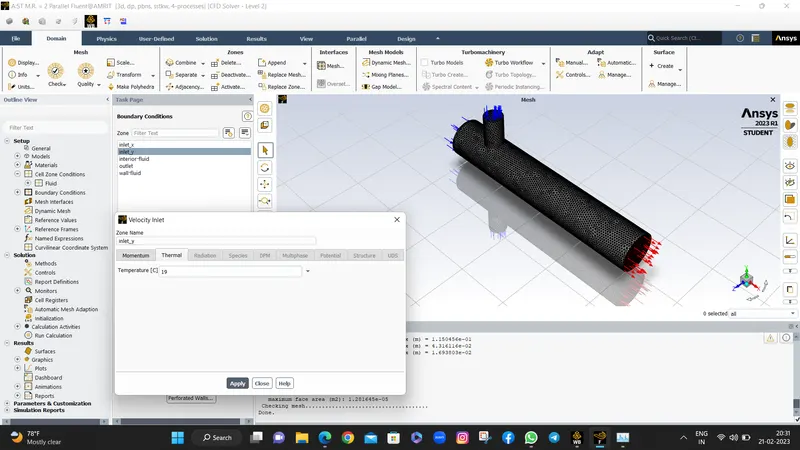
so put this and temp=19 C and then apply and close.

Now click on outlet

It showing pressure-outlet.now click on edit

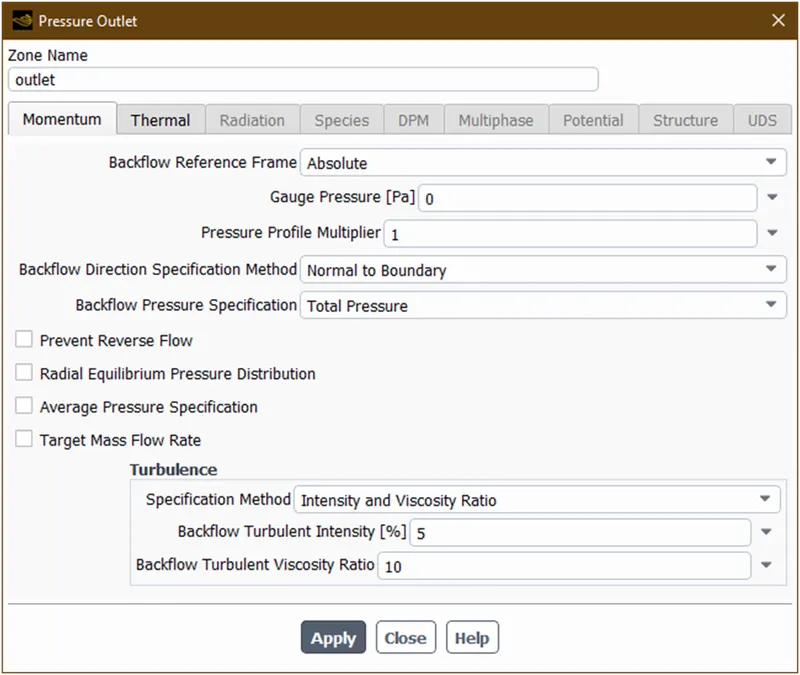
There is no need to change so just apply and close this.and now we have done with boundary conditions.

Now goto solutions->report definitions because we want to findout temps at outlet after calculations

For creating area avg temp.now select the following parameters and give name as shows below.

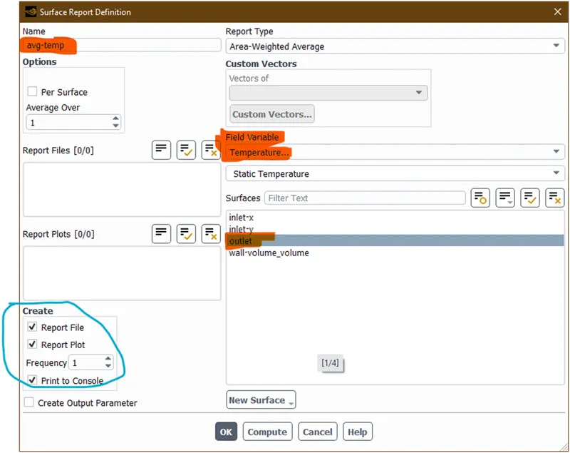
Now we have defined avg-temp report. Similarly define std-deviation temp report

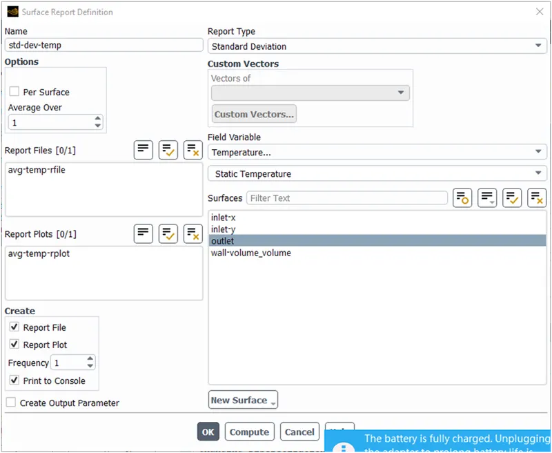
Now close this.now goto solution->initialization

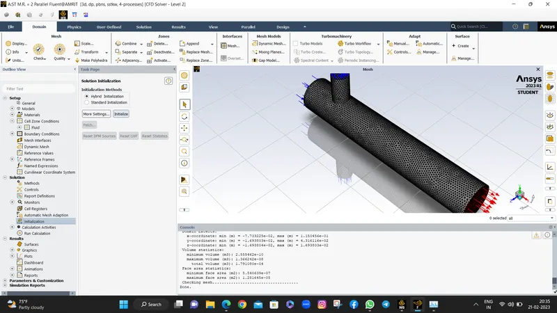
Now goto run calculation

Now give the no.of iterations=100 and scroll down and click on calculate

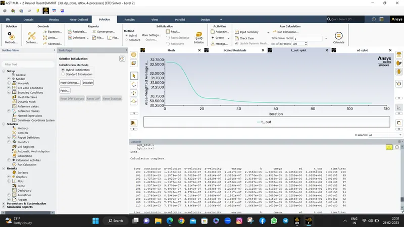
Now wait for calculation to be done.

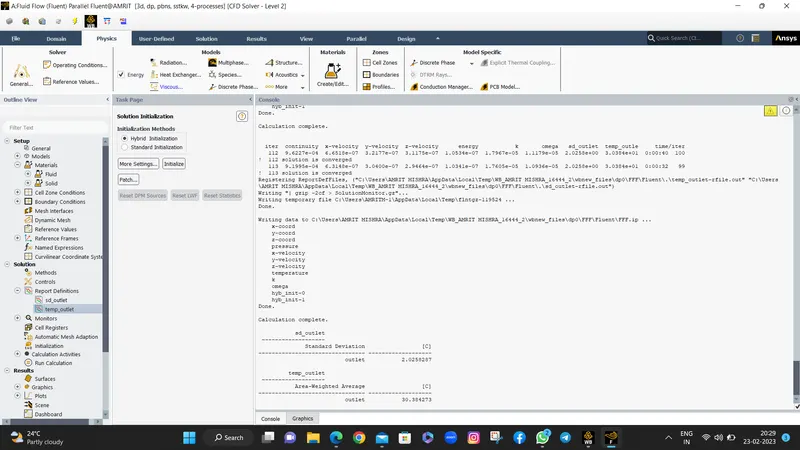
Now its done let see plots.an the message we got as solution has converged.from below plots we can understand the solution is converge on iteration 113.

1. Residual plot

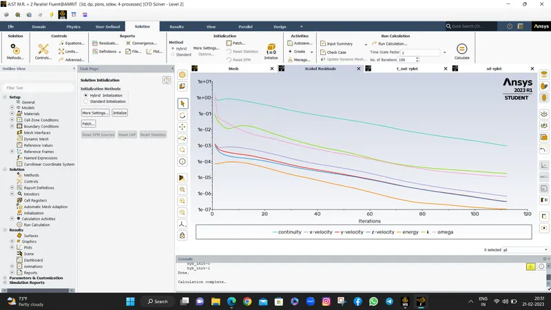
From above graph we can see that the solution is converged at 113 iteration.

2. Area-avg-temp plot

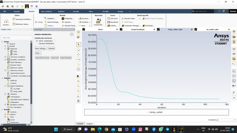
From above graph we can see that the temp graph is almost convergerd , we are getting avg temp at outlet=30.384 C

3. Standard deviation plot

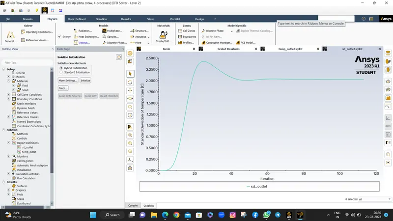
From above graph we can see that std dev temp plot starts converge and std.dev temp=2.025 c.

Now lets plots velocity and temp contours .now close this fluent.

• Goto the results

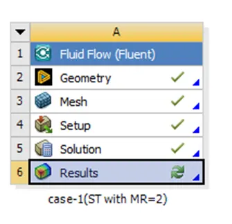
Now enabeled geometry

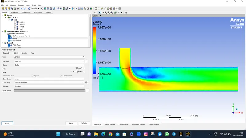
From above velocity contour we can see that inlet-y velocity is not that much in more amount.due to this at upper and lower boundary the velocity of fluid is zero due to Maxwell condition or no slip condition.

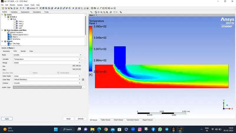
Here the deformation is less at mixing point and also not a good one.from above temp contour we can say that mixing of fluid is not done properly at bottom.so the hot fluid flows and show high temp.

Now similarly we will plot a velocity contour for that just goto color and change the variable as velocity

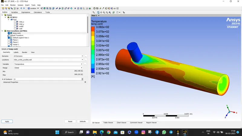
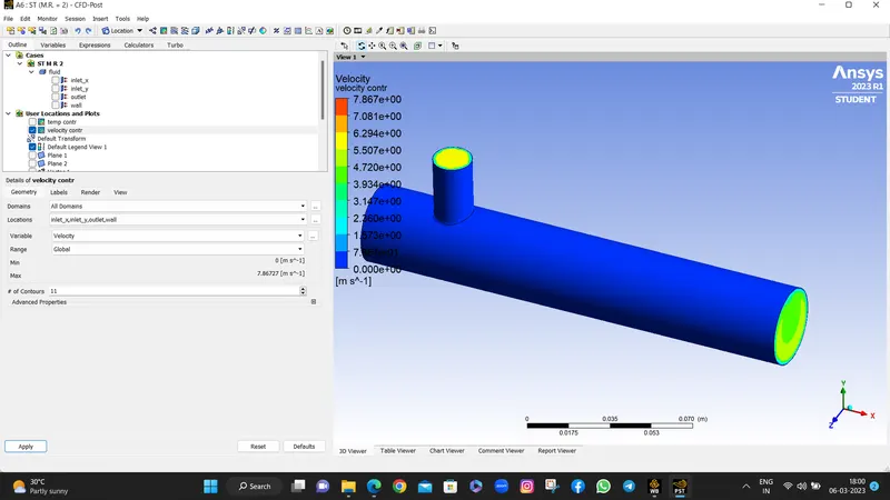
In the above there is Temperature and velocity contour.

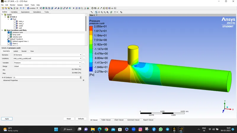
And this the pressure contour with moment ratio= 2 in short tee model.

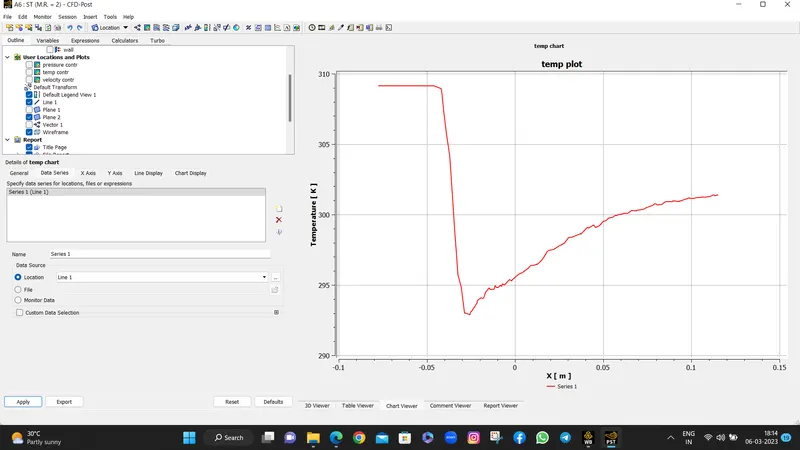
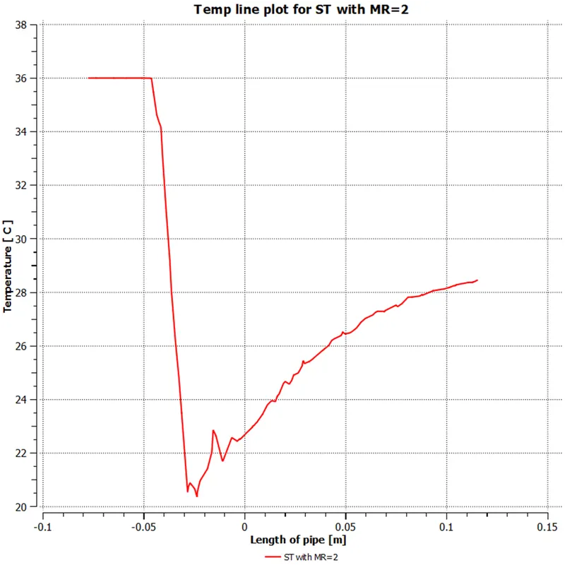
Here the sudden drop is due to cold fluid is entering at that location and after that there is a rise in temp is due to

mixing of fluids taks place and temp of fluid started to stable by exchanging the heat .similarly we are creating the

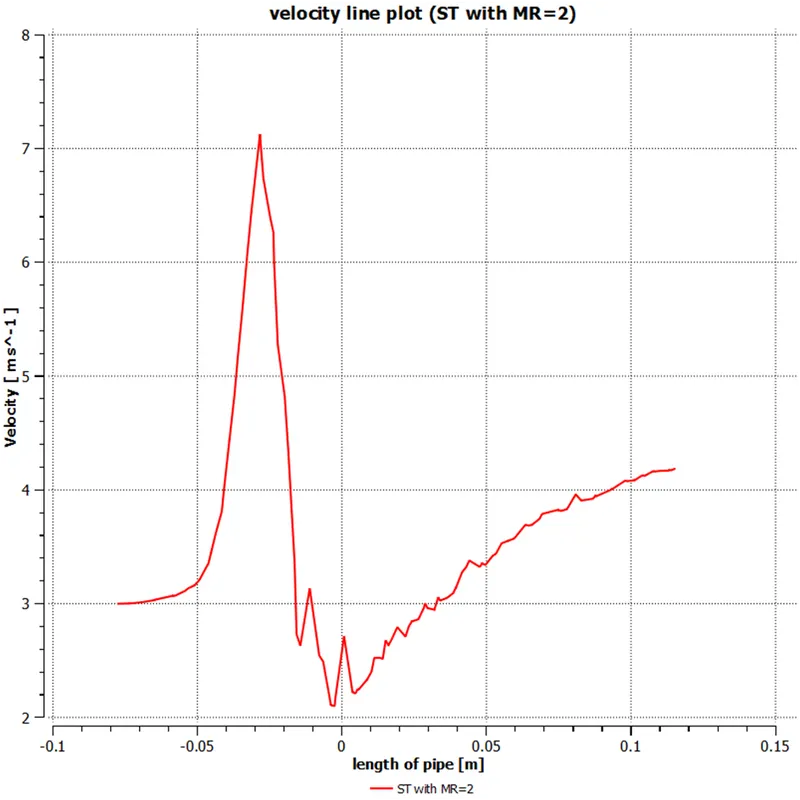
velocity line plot.

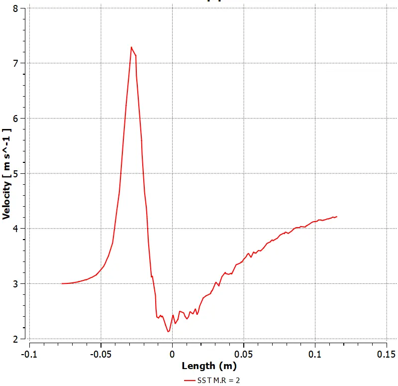
Here the sudden rise is due to the high velocity fluid enters to the pipe at this length of pipe

and as move forward the mixing of fluids with different velocity and gets try to balance as length of pipe increases.

• Now lets calculate avg outlet temp for this case.this can be calculated by using following formula

Here m_hot and m_cold are the mass flow rate and can be obtained directly ansys fluent model For that goto calculators->function calculator -> select variable-> mass flowrate->select location->inlet-x->click on calculate

From here mhot= 0.00330457 [kg s^-1]

Similarly mcold at inlet-y location= 0.00164601 [kg s^-1]

Area Average of Temperature on inlet x

Thot= 36*C

Area Average of Temperature on inlet y

Tcold= 19*C

Now put these values in above eq. and calculate

Tmix(th)= 30.3208*C

And numerically , Area Average of Temperature on outlet

Tmix= 30.384*C

Now by comparing these both are approx equal.

Now we will move for next case.

2. Case-2: Short mixing tee with Momentum ratio=4 :

• Now crate and new project fluent flow

Now right click on first case FF and duplicate it in case-2

• Now open the setup.
• so we duplicate case:1 now i have to just change boundary conditions in this case.

Now apply the boundary conditions.

Now for inlet-y

Here temp=19c and MR=4=Vc/Vh

So, Vc=4*Vh=4*3=12m/s

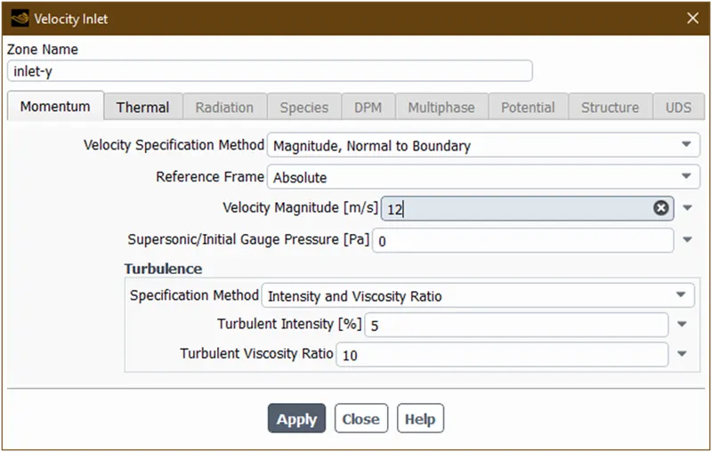
• Here we duplicate the case:1 so we just have to change boundary condition for inlet-y with 12 m/sec velocity magnitude thats it.
• And other configuration is same as it is for in this case.

Now close this and goto solution->initialization->hybrid initialization->initialize

Now goto run calculation and give no.of iteration=100 and hit calculate and wait until calculation done

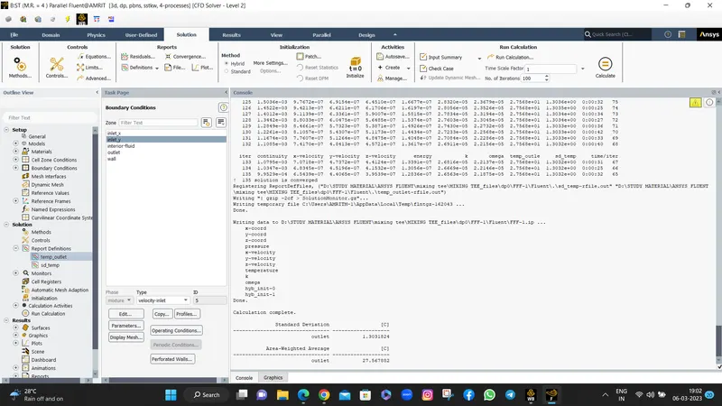
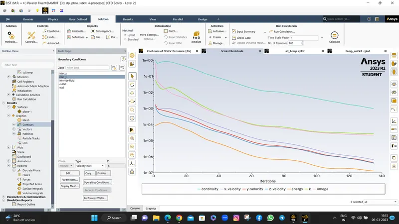
Now calculation done.lets see plots.

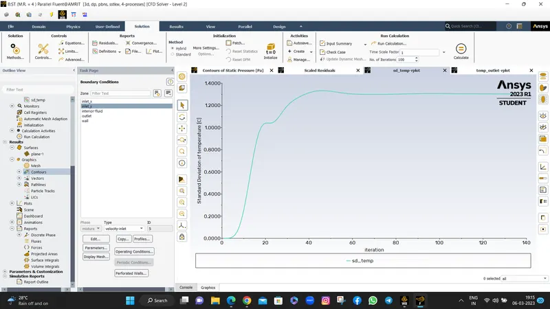
From above graph we can say that std dev temp is almost constant and gives value as 1.3031 C

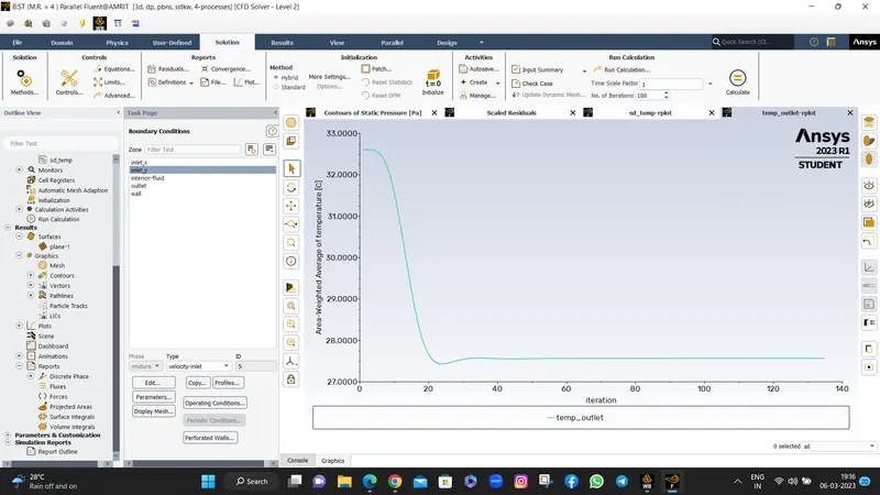
The avg temp is almost constant from 50 iteration and this give value as 27.567 C for this case.

• Lets goto the results to plot temp and velocity contour plots along the cut plane and line plots across the length of pipe in similar procedure.

Now plot the temp and velocity contour plots on plane by creating plane in similar way as mentioned in case-1

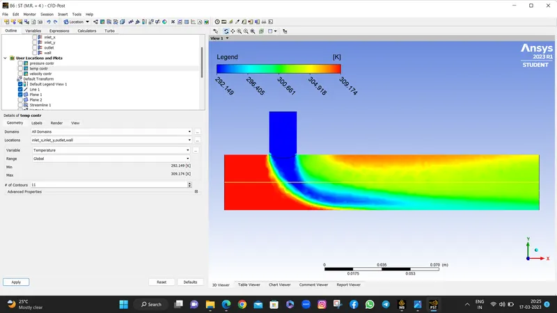
Now here high velocity cold fluid is mixes with low velocity hot fluid. Due to this we can see sudden temp drop at joint and

compareto 1^st case the temp contour is more deviated.and in forward direction the fluid mixes very good.

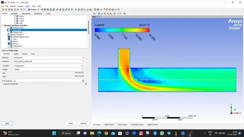
Due to high velocity fluid mixed with low velocity fluid there is sudden change in velocity.and as we see after the t-location

in pipe there is a blue contour shows low velocity is due to sudden entering of high velocity fluid some turbulane created. Lets

plot line plot across the length of pipe.

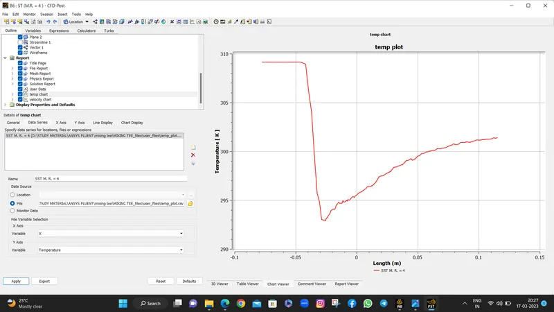
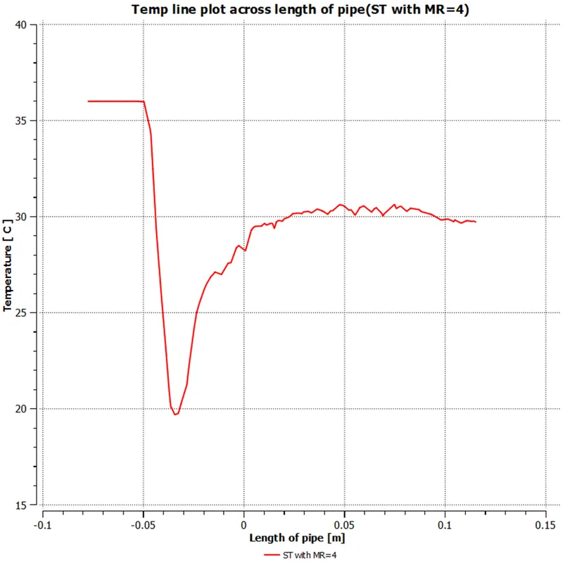
As seen from temp line plot across the length of pipe there is sudden drop in temp due to a cold fluid enters in pipe

after that due to mixing of fluid the temp of fluid increasing as move forward by exchanging the heat between fluids.

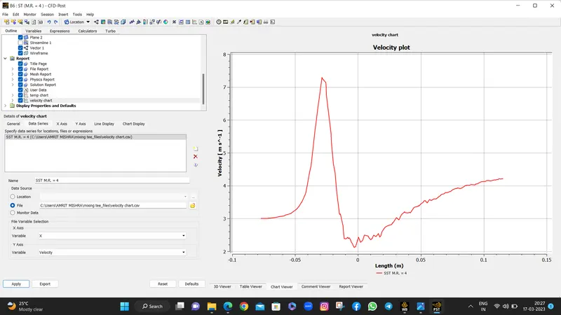
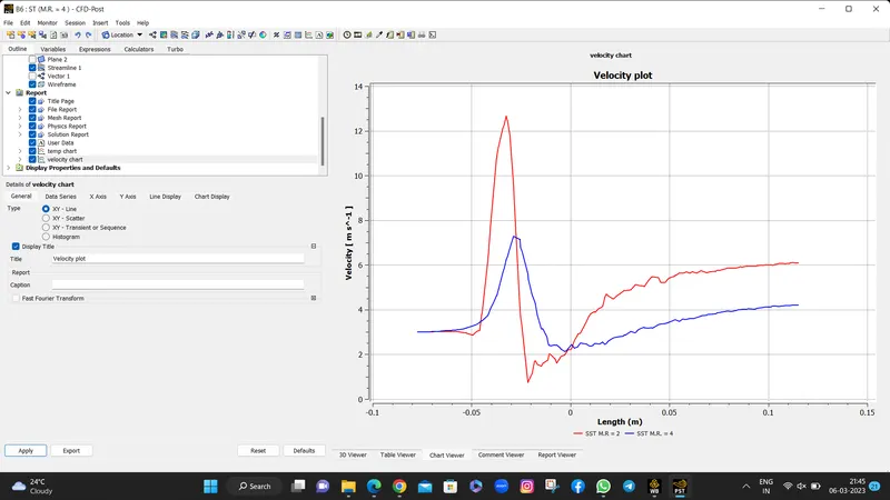
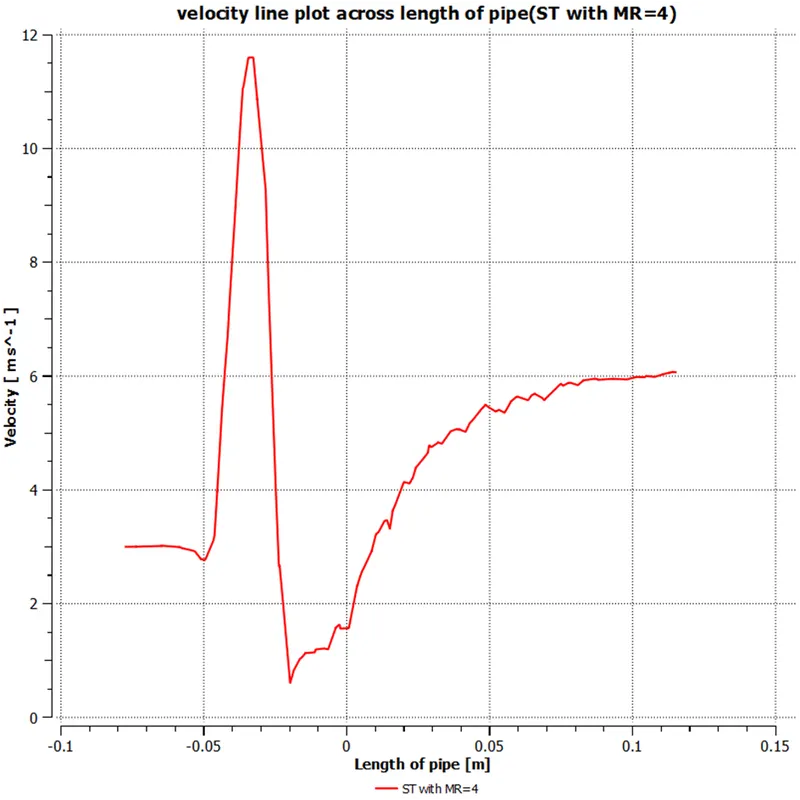
From above graph we can say that sudden increase in velocity at around 0.05m length of pipe is due to high velocity

fluid enters in pipe at this location.and afterward as length of pipe increases 1^st velocity of fluid drops and then started

gradually increases by exchanging the momentum with wach other.

• Let plot comparision plot for short tee

For that goto temp chart

• Now goto data series
• Then click on new
• Give the name and open data points which we have stored sheet and then click on apply

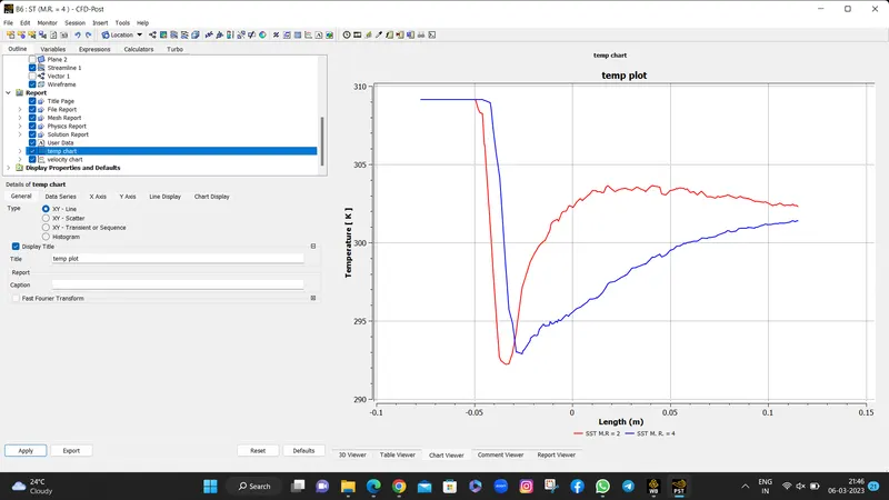
Now its done.Now do similar for velocity also

• Now lets calculate avg outlet temp for this case.this can be calculated by using following formula

Here m_hot and m_cold are the mass flow rate and can be obtained directly ansys fluent model For that goto calculators->function calculator -> select variable-> mass flowrate->select location->inlet-x->click on calculate

• From here mhot= 0.00330457 [kg s^-1]

  Similarly mcold at inlet-y location= 0.00329203 [kg s^-1]

  Area Average of Temperature on inlet x
  
  Thot= 36*C

  Area Average of Temperature on inlet y
  
  Tcold= 19*C

  Now put these values in above eq. and calculate

  Tmix(th)= 27.5161 *C

  And numerically , Area Average of Temperature on outlet
  
  Tmix= 27.5678 *C

By comparing these values our result is validated.

Lets go for next case.

3. Case-3: Long mixing tee with Momentum ratio=2 :

• Create a new projec

• now right click on geometry and import the geometry
• Now browse the long tee model and import
• Now extract the volume
• Now extract the volume
• after this close spaceclaim and open mesh.

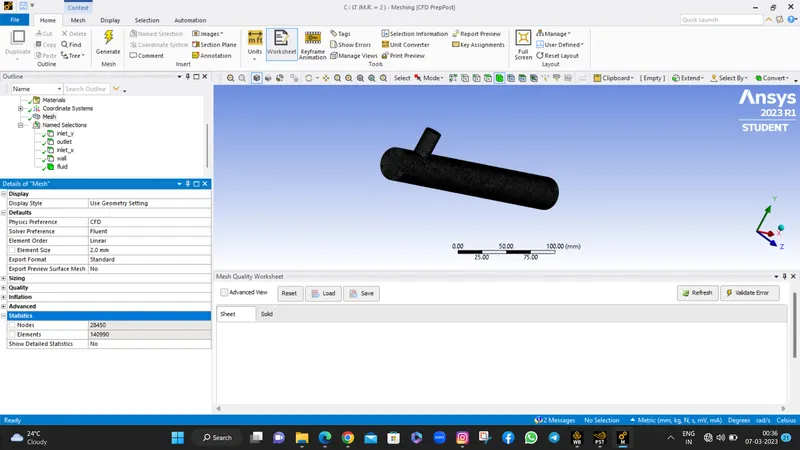
Lets give names as inlet-x,inlet-y and outlet.after that right click on mesh and click on update and then close mesh.

• Goto setup

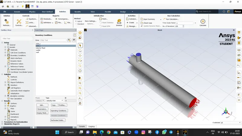
Follow same procedure.setup the models

Apply boundary conditions

Select inlet-x and give V=3m/s and T=36 C

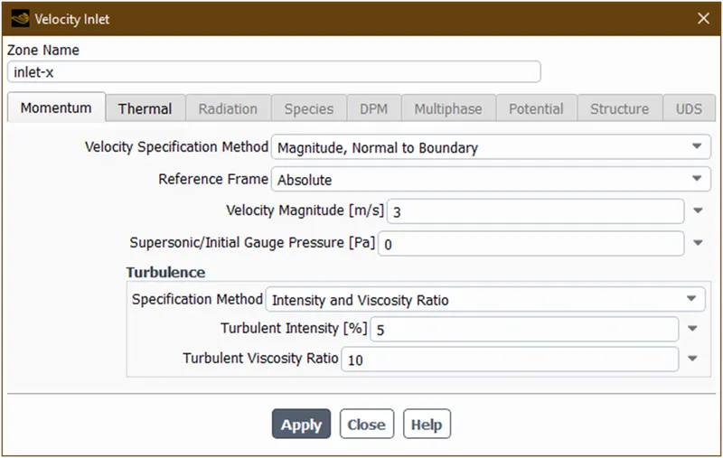
Then click on apply and open inlet-y

Here v=6m/s(because MR=2),T=19 C

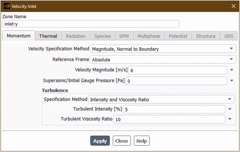
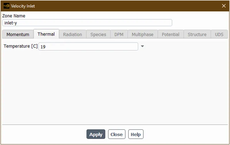
Don’t change anything just close.now goto solutions -> report definition-> create 2 new reports as avg temp and std.dev temp at outlet.

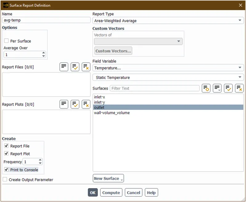
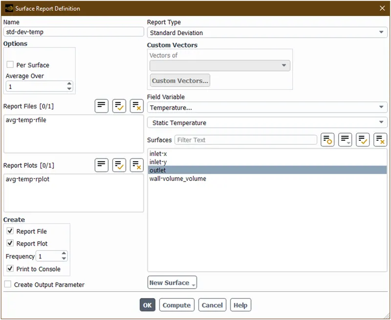
Now initialize solution and run the calculation and wait for calculation complete.

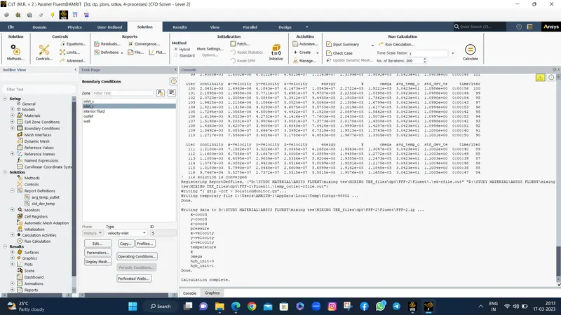
now calculation done.let see residual,area avg temp,std.dev plots

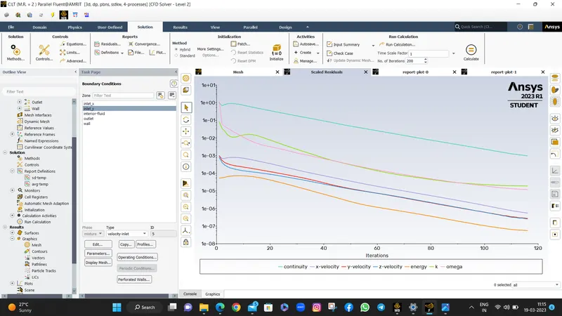
By looking this the solution has converged at 116 iteration.

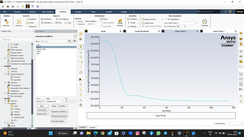
From above graph we are getting avg temp at outlet=30.422 C

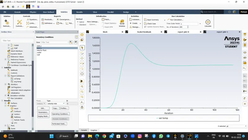
From above graph we are getting std.dev temp at outlet= 1.1004 C

• Lets plot temp and velocity contour plots on cut planes and along and across the the pipe.For that goto results and plot by similar procedure.

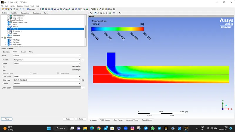
From above temp contour we can say that the cold fluid not mix properly with hot fluid at bottom position due to this at bottom the temp of fluid remains high.

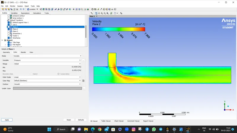
Due to sudden enters of high velocity fluid there is littlebit turbulence created and velocity decreases slightly at after mixing location.

Lets draw a temp and velocity line plots across the length of pipe for this case.

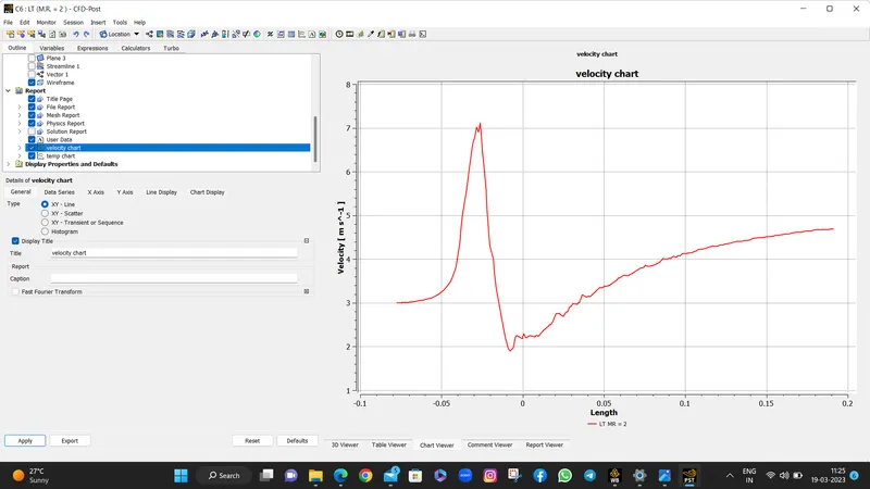
Here there is sudden increase in velocity is due to sudden enters the cold fluid at that location and afterwards velocity

drop and gradually increases due to mixing of fluids take place and also momentum transfer between two fluids.

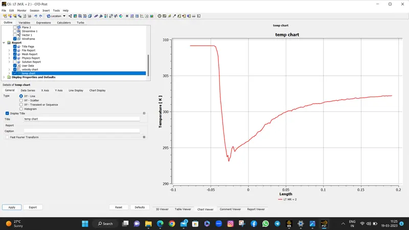
Here there is sudden drop in temp is due to at that location of pipe there is cold fluid enters in pipe and afterwards

there is gradual increase in temp is due to mixing of fluids and exchange of heat between two fluids.

• Lets calculate outlet temp theoretical by using formula

Mass Flow on inlet_x = 0.00330457 [kg s^-1]

Mass Flow on inlet y = 0.00164601 [kg s^-1]

Mass Flow on outlet = 0.00495059 [kg s^-1]

Area Average of Temperature on inlet x = 309.15 [K]

Area Average of Temperature on inlet y = 292.15 [K]

by putting these values we are getting

Tmix= 303.497 k

And by software

Area Average of Temperature on outlet = 303.573 [K]

so it almost equal so our result is validated

Now we will move for next case.

4. Case-4: Long mixing tee with Momentum ratio=4 :

• Open the new project

Now right click on case 3 FF and duplicate it in case-4

• Now open the setup.
• so we duplicate case:3 now i have to just change boundary conditions in this case.

• Now open setup

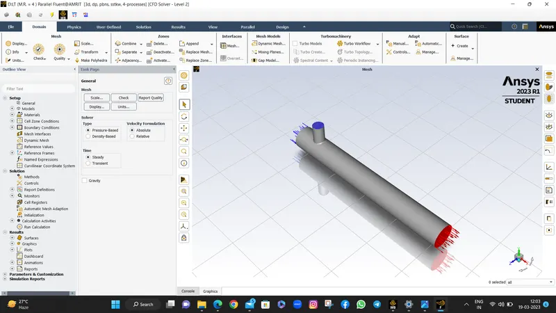
Now apply the boundary conditions.

Now for inlet-y

Here temp=19c and MR=4=Vc/Vh

So, Vc=4*Vh=4*3=12m/s

• Here we duplicate the case:3 so we just have to change boundary condition for inlet-y with 12 m/sec velocity magnitude thats it.
• And other configuration is same as it is for in this case.

Now close this and goto solution->initialization->hybrid initialization->initialize

Now goto run calculation and give no.of iteration=200 and hit calculate and wait until calculation done

Lets see plots

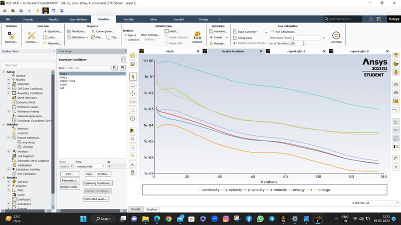
From this graph we can see that the solution has been converged at 137 iterations.

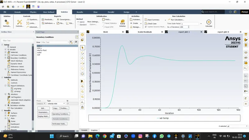
From above graph std dev temp= 0.53823292 C

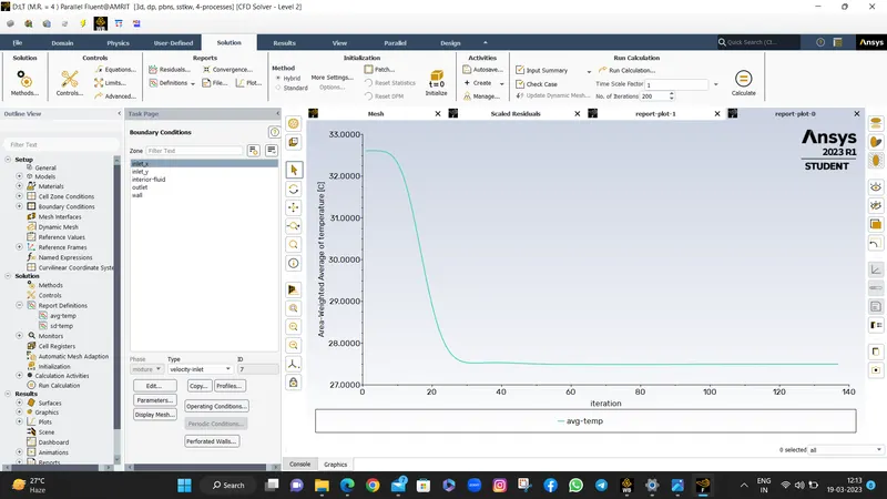
From above graph we can see that area avg temp get converged= 27.498258 C

• now lets plot temp and velocity contour plots by same procedure.for that close fluent and goto results

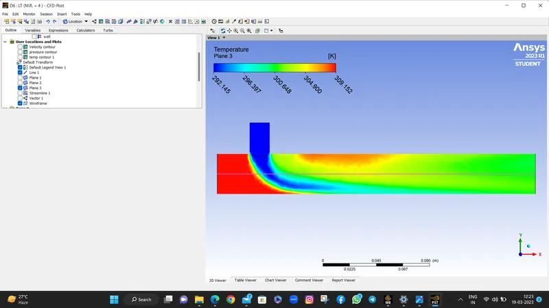
From above graph we can see that there is a diffusion of temp contour of cold fluid and by seeing this the mixing of fluid is very well .

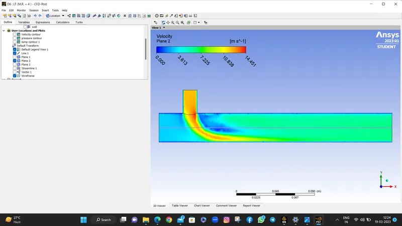
By seeing this velocity contour there is more diffusion of high velocity and less turbulence after T-joint.

Lets plot temp and velocity line plots

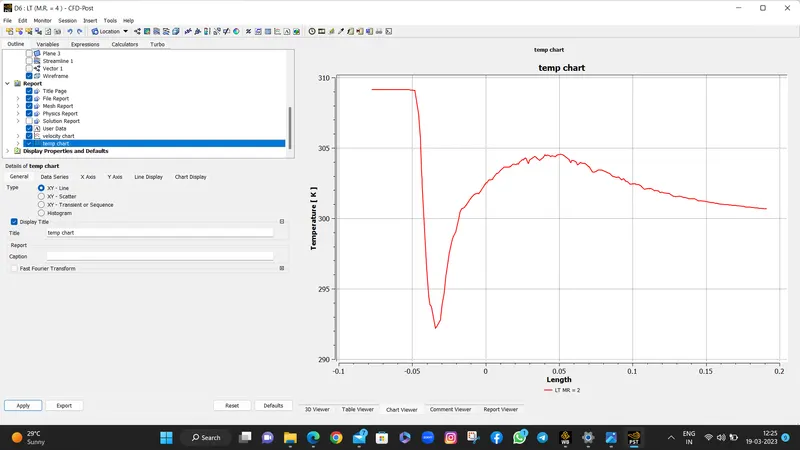
There is sudden drop of temp is due to cold fluid enters in a pipe at this section and afterward there is a

gradually increase in temp is due to mixing of fluids and exchanging the between them.

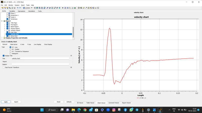
There is sudden rise in velocity is due to high velocity fluid enters in pipe at this location.and after that mixing of

fluid takes place due to this the momentum transfer takes place between fluids.

• lets find out avg temp theoretically by using same formula

Mass Flow on inlet x = 0.00330457 [kg s^-1]

Mass Flow on inlet y = 0.00329203 [kg s^-1]

Mass Flow on outlet = 0.0065966 [kg s^-1]

Area Average of Temperature on inlet x =309.15 [K]

Area Average of Temperature on inlet y =292.15 [K]

Tmix = mh * Th + mc * Tc/(mh + mc)= 300.666 [K]

And by numerically or by software

Area Average of Temperature on outlet = 300.648 [K]

by comparing these ywo values our result is validated.

That conclude all . lets see results and conclude it.

Results :

1. Velocity and temperature contour plots on the cut planes along and across the pipe :
   1. Case-1 :short mixing tee with momentum ratio=2 :

Here at bottom of the pipe the mixing is not done properly due to this the hot air remains and temp is high.

due to mixing of fluid after t-section turbulence was created and velocity decreases near to T-section.

b. Case-2 : short mixing tee with momentum ratio=4 :

Compared to previous case we can see that as velocity of cold fluid is 2times the previous case due to this the mixing

of fluids is done properly and temp distribution is more efficient to previous case.here at upper surface there is not a

good mixing of fluid taks place so it shows high temp.

As we can see that in above contour as velocity is 2 times to the previous case there is more turbulence created near

to the inlet-y and velocity deformation is more.

Case -3 : long mixing tee with momentum ratio=2 :

As we see in this temp contour there is not properly mixing done at bottom. But compared to sort tee the temp

distribution is looks good.

As we seen in above velocity contour there is more deviation of cold fluid compared to previous two cases and there

is less turbulence near to cold fluid inlet section.

d. Case-4 : long mixing tee with momentum ratio = 4:

Here due to high velocity the cold fluid is mixes with hot fluid very quickly and temp distribution takes properly but

at upper side there is not a good mixing of fluid so heat transfer between fluids is not proper. again at upeer surface

near to inlet-y there is not a good mixing of fluid takes place.so som hot fluid traces shows.

At boundary there is very low velocity but due to high velocity of cold fluid the deformation is more and gets steady

state very quickly.

2. Velocity and temperature line plots along and across the length of the pipe :
   1. Case-1 :short mixing tee with momentum ratio=2 :

b. Case-2 : short mixing tee with momentum ratio=4 :

C. Case -3 : long mixing tee with momentum ratio=2 :

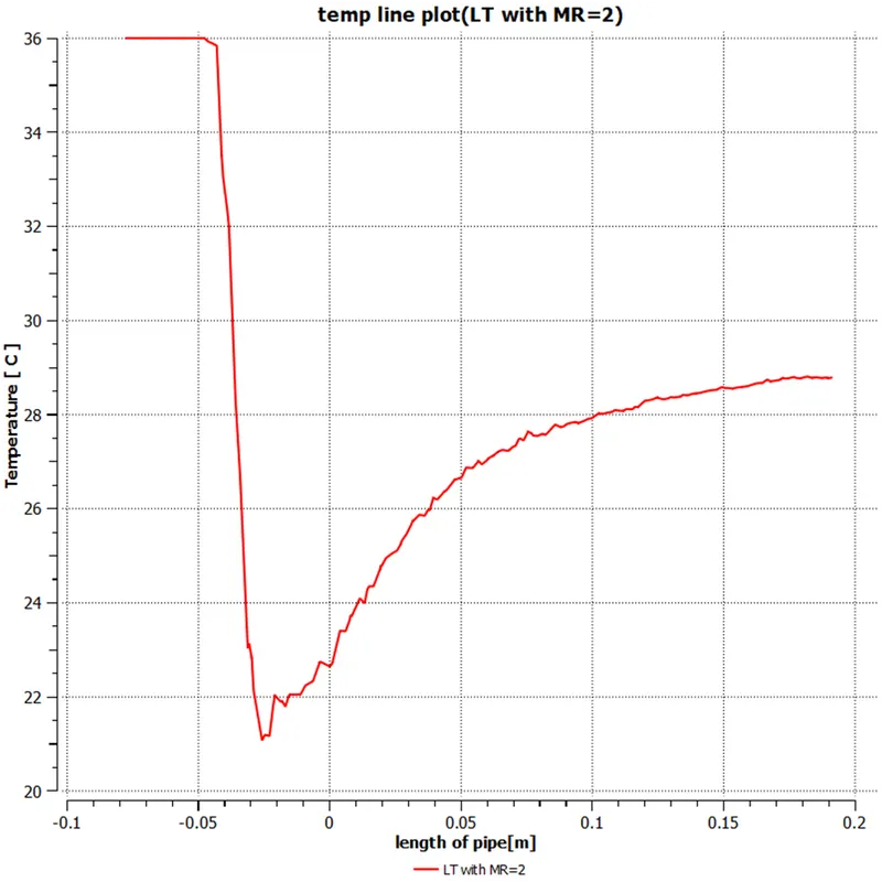
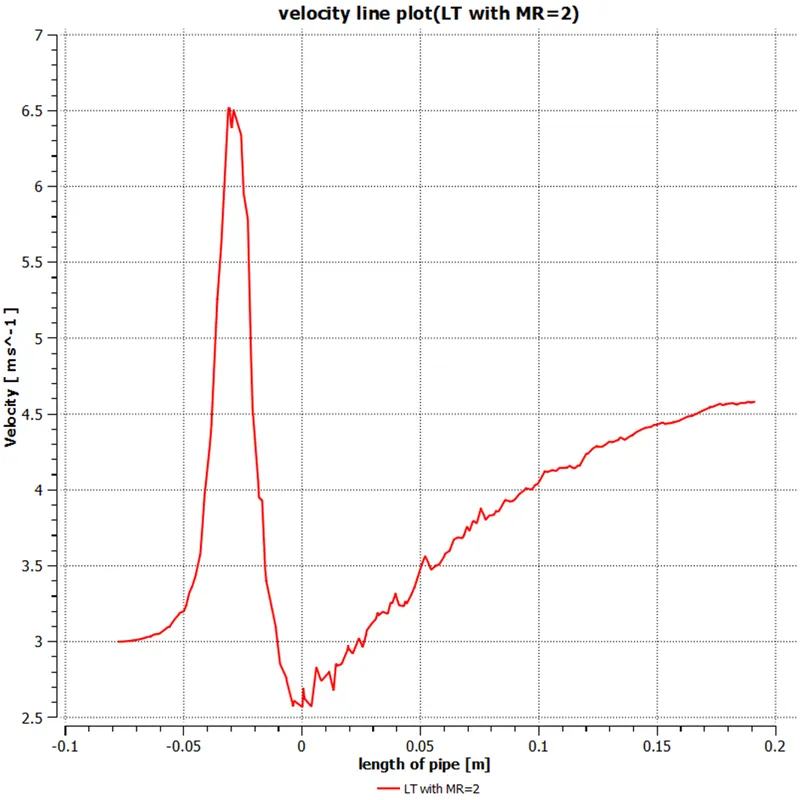
D. Case-4 : long mixing tee with momentum ratio = 4:

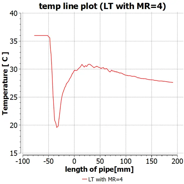
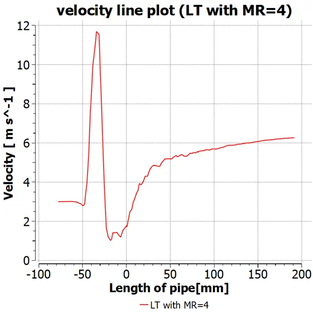
3. Comparison of plots of cases :

1. Comparison of temp and velocity line plots for Short tee

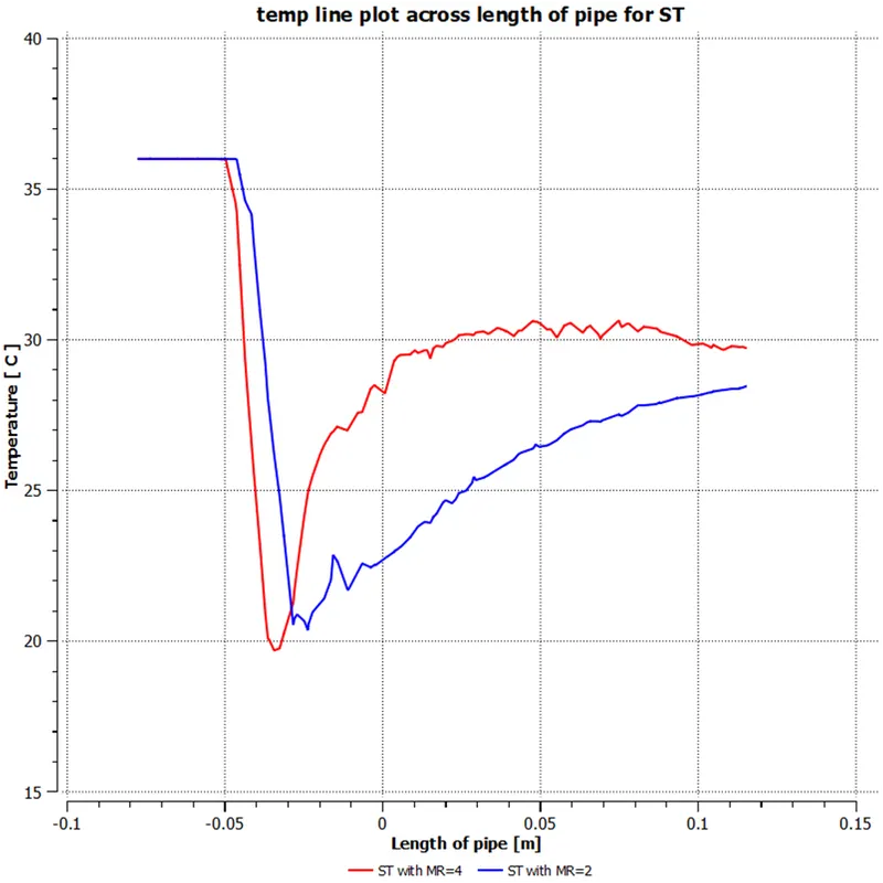
In this case as MR increases temp curve also gets stepper. after inlet-y section the temp gradually increses.at the center of pipe the temp gets little bit uniform/constant.

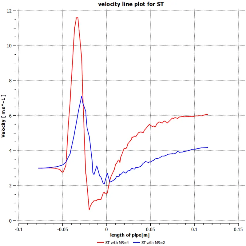
As MR increases the steepness of curve at inlet increases.

b. Comparison of temp and velocity line plots for long tee

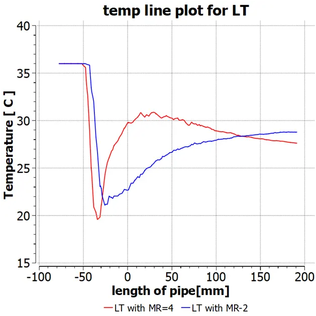
In this case as MR increases the outlet temp decreases.after ceratain length of pipe the temp decreases for LT with MR=4.

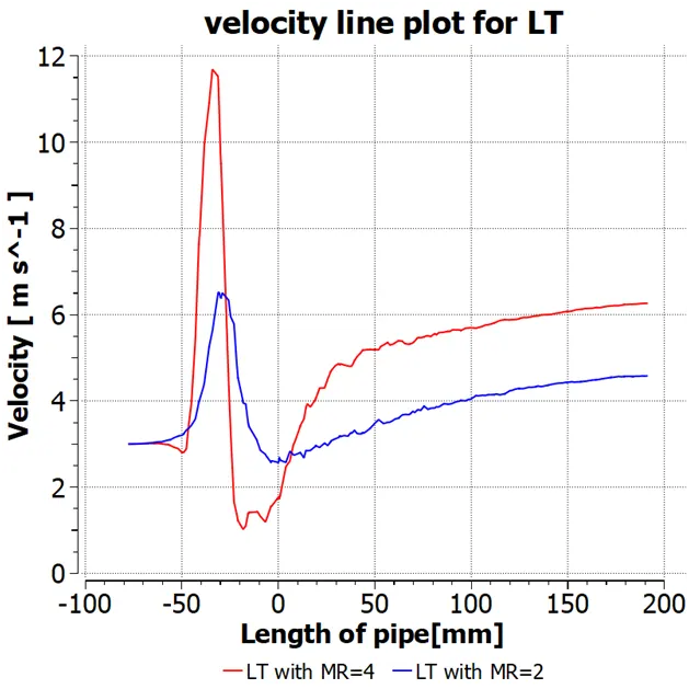
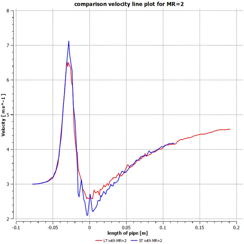
c. Comparison of temp and velocity line plots for MR=2 :

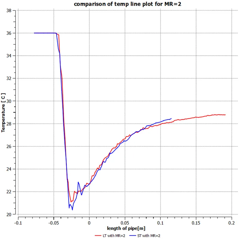
as length of pipe increases there is no change in temp line plot for same MR. the plots gets coincide.

d. Comparison between temp and velocity line plots for MR=4 :

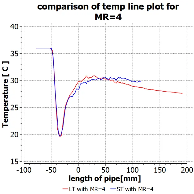
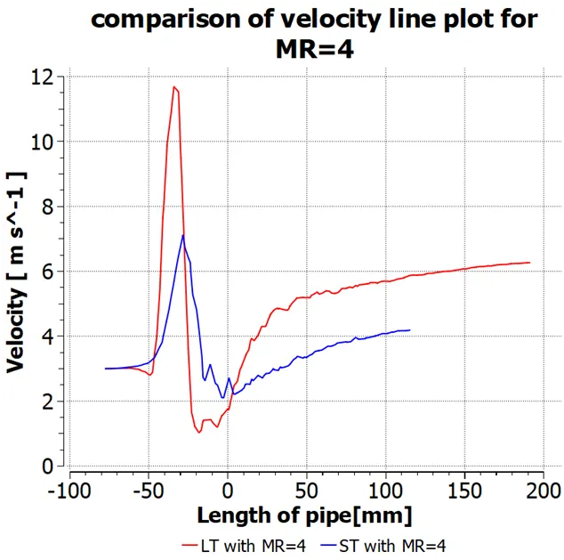
4. Numerically comparision of outlet temp

Sr no	Cases	Avg Outlet temp(K)			Cell count	No.of Iteration for convergence of solution
		Theoretically		Numerically
1	ST with MR=2	303.470	303.534		106253	113
2	ST with MR=4	300.666	300.717		106253	135
3	LT with MR=2	303.497	303.573		140990	114
4	LT with MR=4	300.666	300.648		140990	137

Conclusion :

• From result1 i.e. from temp and velocity contours we can conclude that as velocity increases the deformation of temp and velocity is more and there is good mixing of fluids and heat transfer.

• From result 2 i.e.from temp line plot and velocity line plot we can conclude that at inlet section of cold fluid there is a sudden drop in temp and afterwards as flow moves along a length of pipe temp gradually increases and mixing of fluid takes place and temp reaches steady state. As MR increases the curve becomes more steeper.Now talking about velocity line plot as high speed velocity fluid enters into the pipe there is sudden increase then falls at that cross-section in velocity and as mixture moves forward along the length of pipe the mixing of fluid takes place and there is a gradually increase in velocity and reaches the steady state .

• From result-3 we can say that for same MR as we increase the length of pipe there is no difference in temp and velocity line plots across the length of pipe.

• From result-4, we can say that our results are validated with theoretical results.