Week 1- Mixing Tee
AIM
To study effect of mixing in respect to length of the pipe and temprature distributuion and then perform a mesh independent study on the effect of the results.
Steps involved:
1. Geometry Preparation
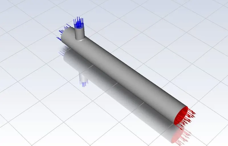
Prepare the geometry by extracting the geomerty where the fluids will be coming in contact with the walls.
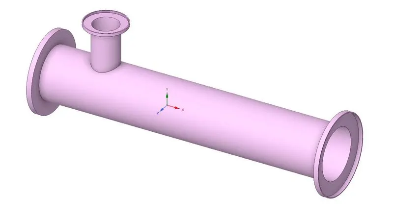
Launch spaceclaim for volume extraction and use the volume extract command from prepare tab to create the requried geometry and suppress the full geomerty so that while doing analysis it will not be taken into account. Now close the spaceclaim
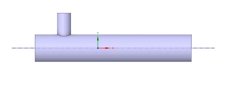
2. Meshing the Fluid volume
NOw double click the mesh function and first give names to all relevant surfaces as follows:
Inlet y - Hot air coming inlet
Inlet x - Cold air coming inlet
Outlet - Outlet after the mixing
Walls - Surfce of the pipes
Now after this with the default mesh settings, genarate mesh.
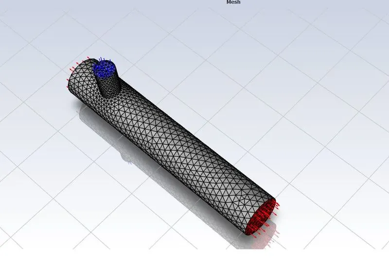
Make sure the mesh quality is not than 5 %.
Now close the mesh and right click the mesh and click update.
3. Setting up the Simulation
Open the setup which will open the Ansys Fluent.
Now make sure the setup is steady state pressure based model with absolute velocity formulation.
As we are solving for temprature make sure we tick the energy equation.
As the flow can be turbulent, we will run simulation with both K-epsilon model and K-omega model and will see the effects in the results.
Now add the material and select air as the material.
Now assign the boundary conditions.
Go to cell zones and click on Volume then click edit and make sure it is air.
Now click boundaries and click the inlet x. Now click edit ans put the velocity as 3m/s and set the temprature as 36C
Now click the inlet y and click edit. We will run with momentum ratio 2, 4 that means with the velocity of 6 and 12m/s and temprature as 19C.
Now set the outlet boundary condition as pressure outlet with a gauge pressure of 0Kpa. Now we will define the parameters to see the outlet conditions such as area weighted average of temprature and standard deviation of the temprature at the outlet.
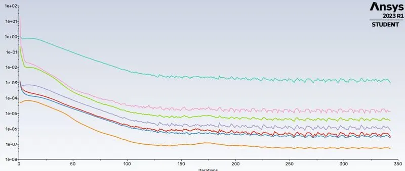
After setting up the boundary condition, click on initialize and set the number of iteration as 250 and click calculate which will run the simulation.
So here we will be doing a few different analysis with various boundary conditions and tubulence model to study the effect of each parameters on the results.
Results
1. Case 1 with K epsilon and momentum ratio 3
Option 1 with coarse mesh
Here we used the ansys generated mesh size and used K epsilon Turbulent model
Inlet conditions are :
Inlet x - 3m/s and 36C
Inlet y - 6m/s and 19C
Outlet - Presuure outlet at 0 Pascal Gauage pressure
Results to plot:
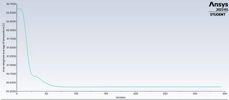
Standard deviation of temprature, Area weighted average of temprature.
Outcomes:
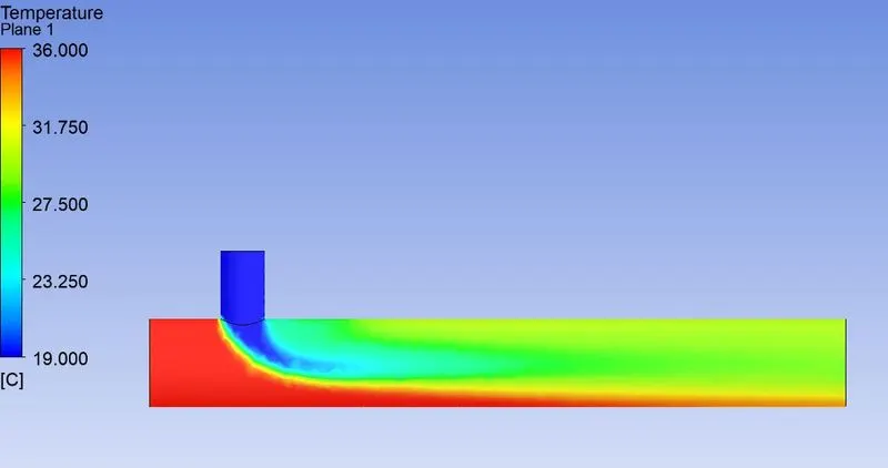
As standard deviation is around 1.7 the temprature mixing is not very uniform.
As the mesh is not very fine the solution looks diffused at the mixing area.
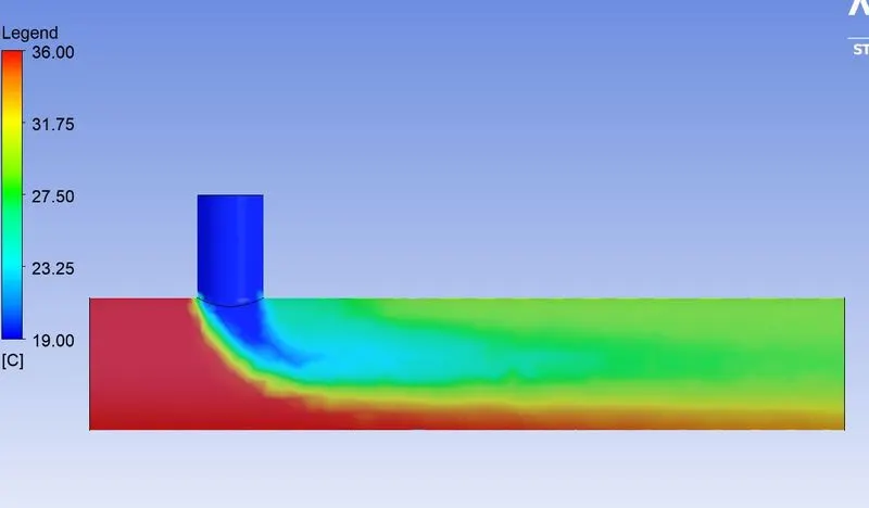
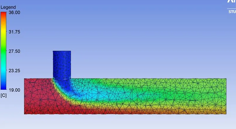
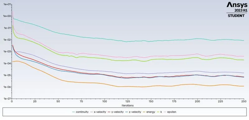
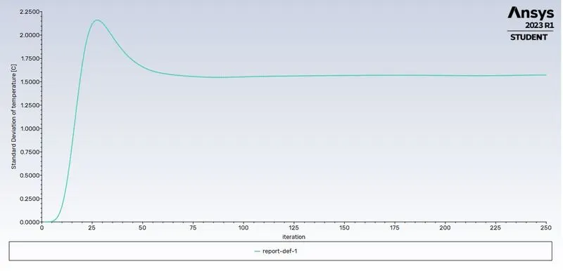
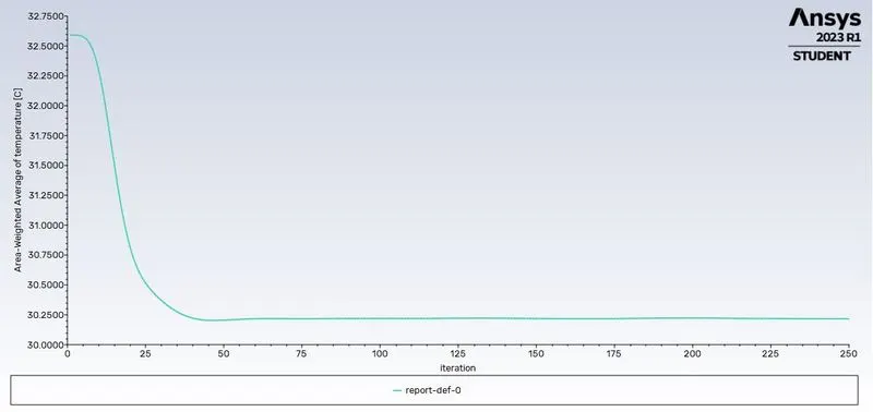
As the momentum ratio is only 2, the mixing is not proper and the temprature did not come down much at the outlet.
We can see the temprature at the outlet is close to 30.2C
2. Case 1 with K epsilon and momentum ratio 4
Option 1 with coarse mesh
Here we used the ansys generated mesh size and used K epsilon Turbulent model
Total elements 12780
Inlet conditions are :
Inlet x - 3m/s and 36C
Inlet y - 12m/s and 19C
Outlet - Presuure outlet at 0 Pascal Gauge pressure
Results to plot:
Standard deviation of temprature, Area weighted average of temprature.
Outcomes:
As standard deviation is around 1.7 the temprature mixing is not very uniform.
As the mesh is not very fine the solution looks diffused at the mixing area.
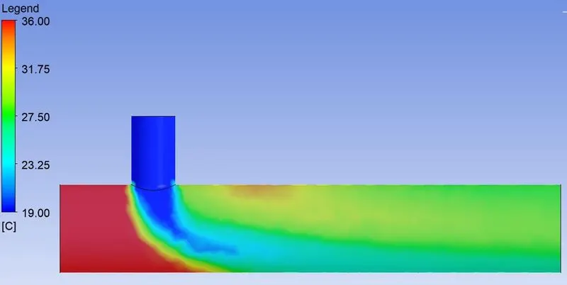
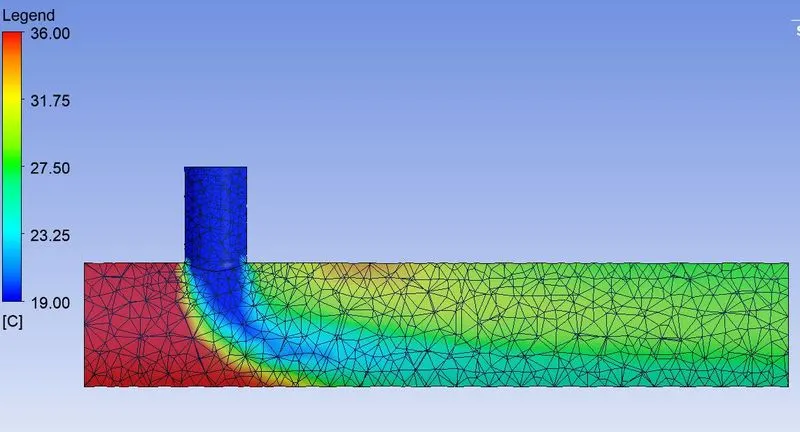
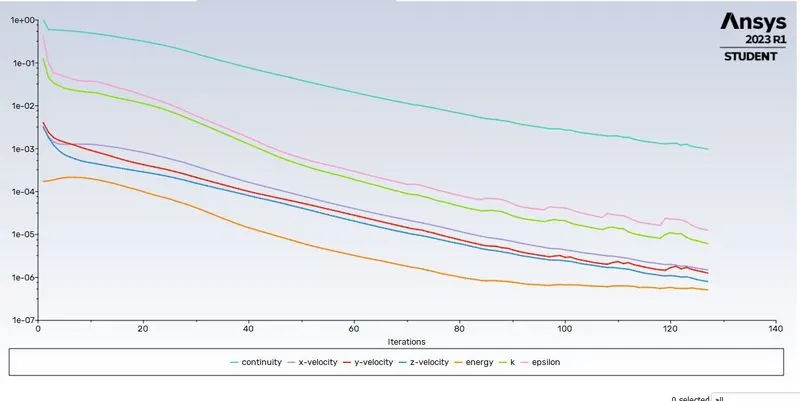
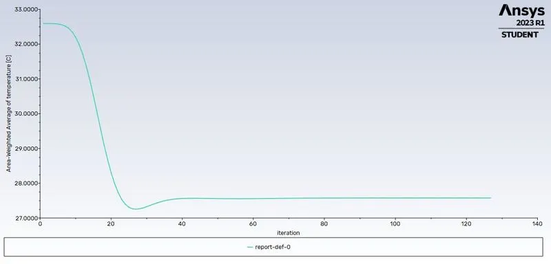
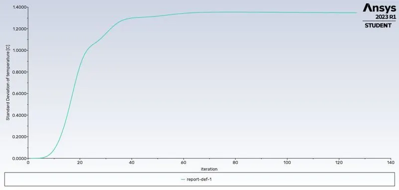
As the momentum ratio is 4, the mixing is more effective and the temprature did not come down much at the outlet.
We can see the temprature at the outlet is close to 27.5C
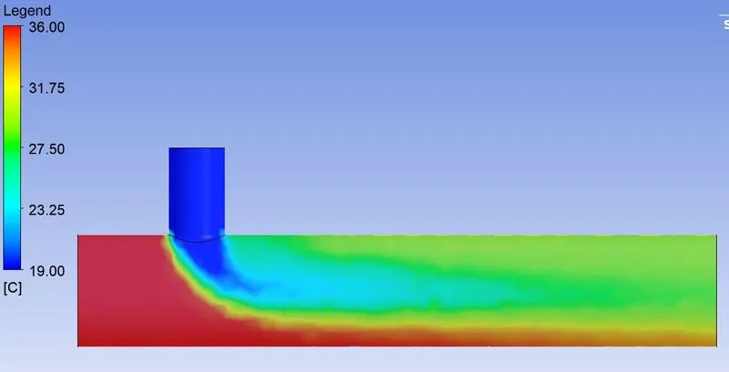
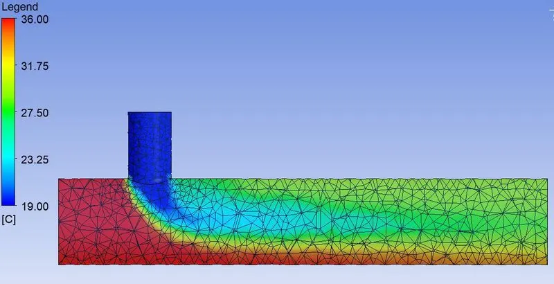
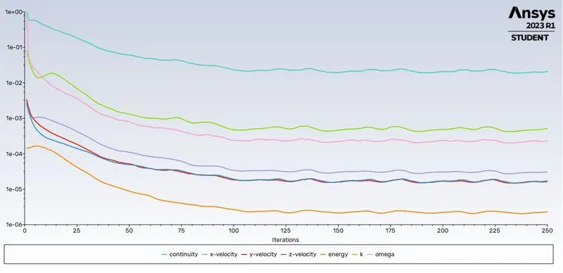
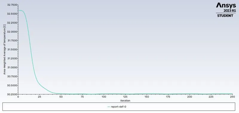
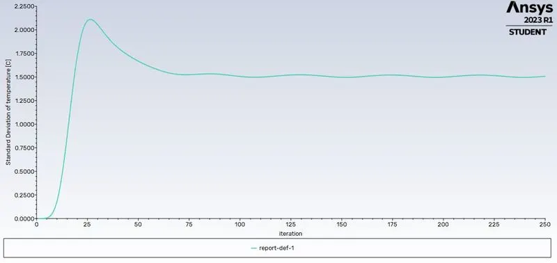
3 Case 1 with K Omega SST and momentum ratio 2
Here we used the ansys generated mesh size and used K epsilon Turbulent model
Total elements 12780
Inlet conditions are :
Inlet x - 3m/s and 36C
Inlet y - 6m/s and 19C
Outlet - Presuure outlet at 0 Pascal Gauge pressure
4 Case 1 with K Omega SST and momentum ratio 4
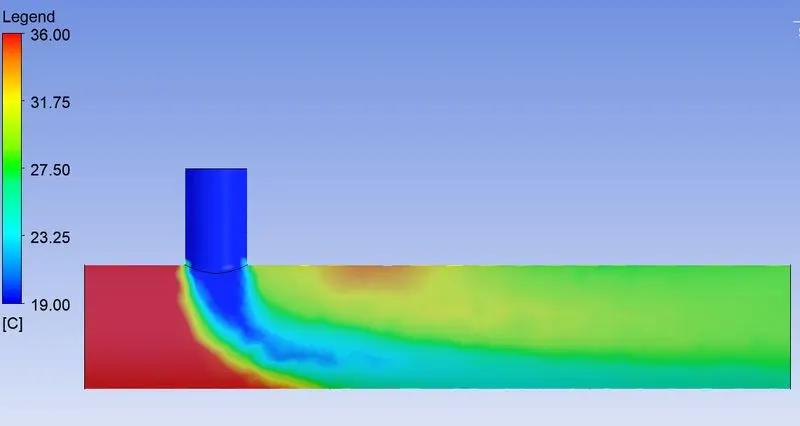
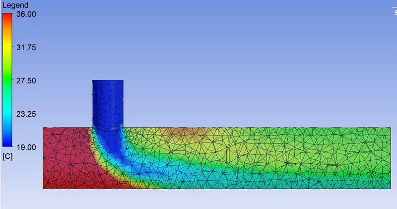
Here we used the ansys generated mesh size and used K epsilon Turbulent model
Total elements 12780
Inlet conditions are :
Inlet x - 3m/s and 36C
Inlet y - 12m/s and 19C
Outlet - Presuure outlet at 0 Pascal Gauge pressure
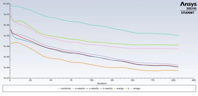
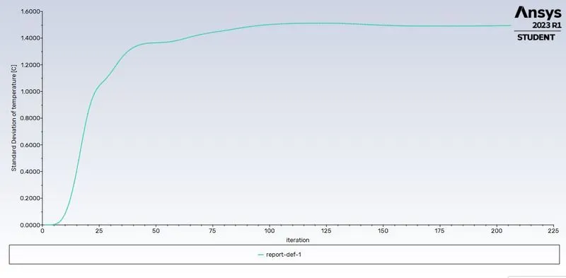
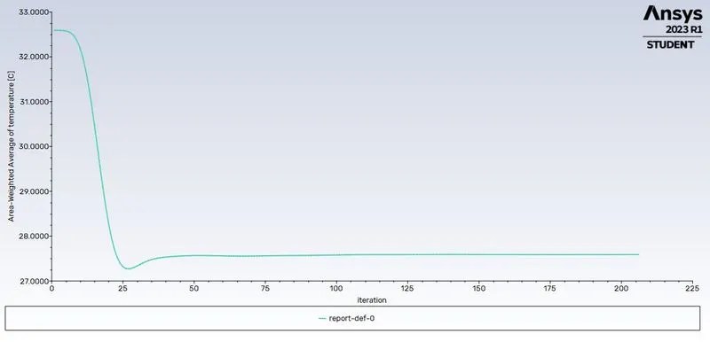
Comparison
Here we will compare the results for both tubulent models K epsilon and K omega to understand which one is better for our further analysis.
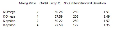
From the above table it is clear that resulting outlet tempratures are similar in both cases but the standard deviation is bit different.Also we can notice the number of iteration required to converge the results are less for the K epsilon model.Also K Omega model is more accurate in capturing the details near the wall whereas K epsilon is good at regions away from the wall. Due to this resons we will be using the K epsilon model for our further analysis.
5 Case 2 with K Epsilon and momentum ratio 4
Here we used the ansys generated mesh size and used K epsilon Turbulent model
Total elements 140990
Inlet conditions are :
Inlet x - 3m/s and 36C
Inlet y - 6m/s and 19C
Outlet - Presuure outlet at 0 Pascal Gauge pressure
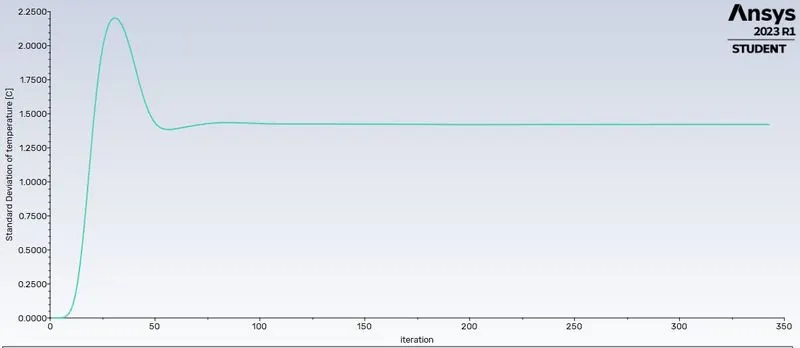
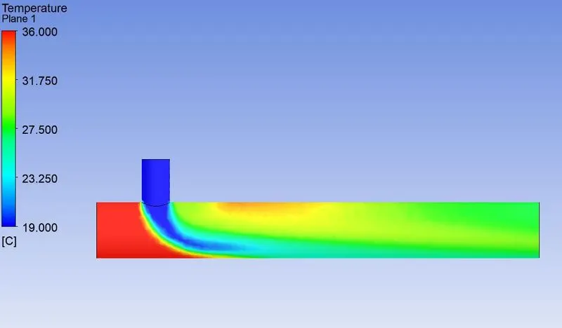
6 Case 2 with K Epsilon and momentum ratio 4
Here we used the ansys generated mesh size and used K epsilon Turbulent model
Total elements 140990
Inlet conditions are :
Inlet x - 3m/s and 36C
Inlet y - 12m/s and 19C
Outlet - Presuure outlet at 0 Pascal Gauge pressure
Results
Results from the analysis of case for using K epsilon turbulence are as follows:

Conclusion:
1. Reducing the mesh size will give us a more refined reprasenttion and results.
2. K epsilon turbulence model is better for analysis away from the wall and K omega are good near to the walls.
3. As the momrntum ratio increases, proper mixing happens.