Week 1- Mixing Tee

Aim

Set up steady-state simulations to compare the mixing effectiveness when hot inlet temperature is 36C & the Cold inlet is at 19C.

• Case 1 A: Short mixing tee with a hot inlet velocity of 3m/s. Momentum ratio of 2
• Case 1 B: Short mixing tee with a hot inlet velocity of 3m/s. Momentum ratio of 4
• Case 2 A: Long mixing tee with a hot inlet velocity of 3m/s. Momentum ratio of 2
• Case 2 B: Long mixing tee with a hot inlet velocity of 3m/s. Momentum ratio of 4

Momentum ratio = velocity at cold inlet / velocity at hot inlet

Part 1: Use the k-epsilon and k-omega SST model for the first case and select the best suitable model for further cases

Part 2: Perform Mesh independence study for any one case.

Part 3: In a table, compare the following values from the 2 cases.

• Cell count
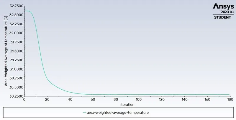
• Average outlet temperature
• Number of iterations for convergence

Expected results:

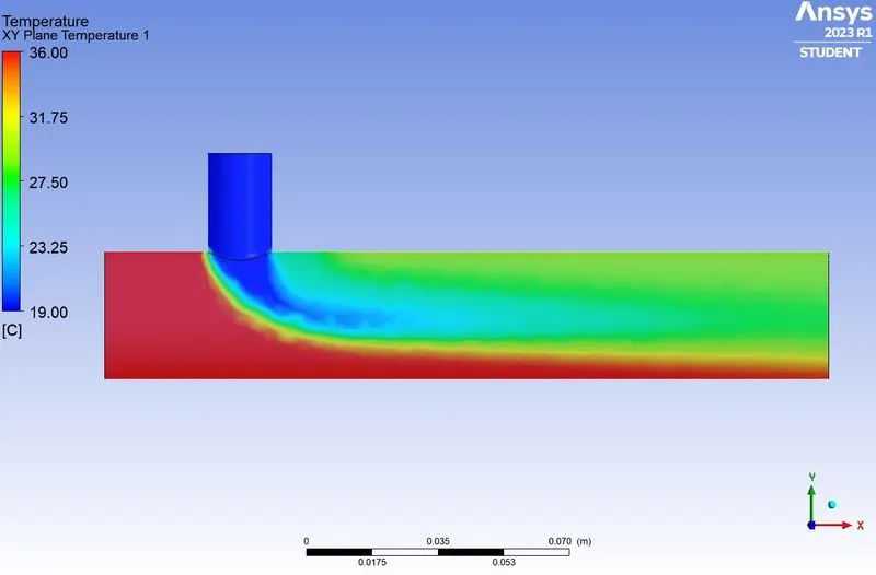
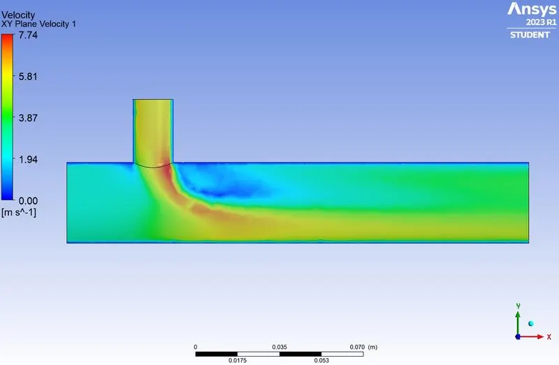
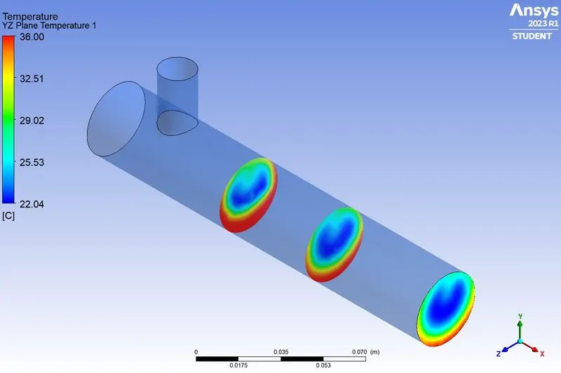
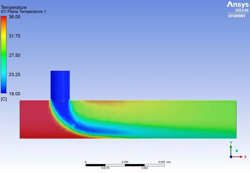
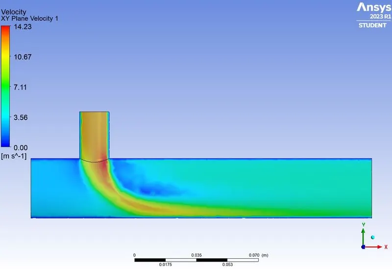
• Velocity and temperature contour plots on the cut planes along and across the pipe (from Part 3)
• Velocity and temperature line plots along and across the length of the pipe (from Part 3)
• Discuss the effect of length and momentum ratio on results.

Introduction

Computational fluid dynamics is a branch of fluid mechanics, which uses mathematics and physics through a computational software to solve and predict fluid dynamics in a system. Various governing equations like conservation of momentum – Navier stokes equation, conservation of energy etc are used to predict the fluid flow phenomena. 

The software used for CFD in this study is Ansys Fluent. Ansys Fluent is a well-known tool in CAE domain.

In this study we are going to analyse the effectiveness of a mixing tee, which is a pipe geometry that facilitates mixing of two fluid streams. We will use two different mixing tee varying in length and analyse the effect of length and momentum ratios on the mixing effectiveness of the two fluid streams.

Theory

The function of Mixing Tee is to facilitate mixing of fluid streams to get the desired level of a particular quantity of interest at the outlet. When Hot air and cold air streams with different temperatures and velocities are going to mix in a mixing tee, the temperature at the outlet will be somewhere between the two inlet streams. By controlling the velocity of cold air stream we can control the temperature at the outlet.

This principle is used widely to achieve required fluid temperatures in cooling systems.

Solution and Modelling approach

General Simulation approach

 

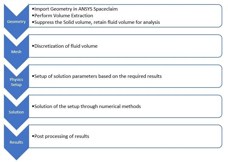
Approach for current Study

 

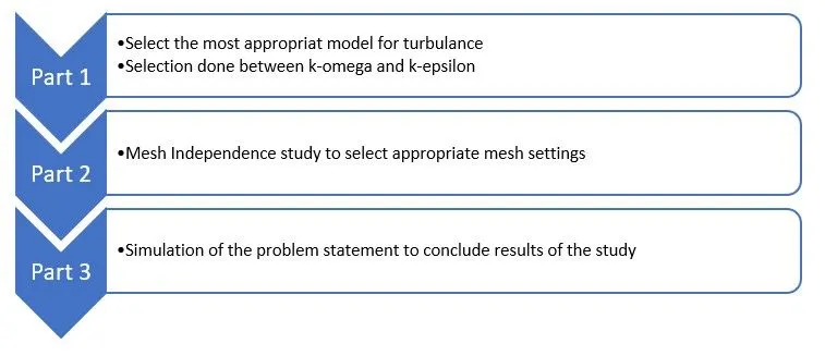
Procedure

Part 1:

First part of this study involves selection of the best method to ensure convergence of the solution by studying two turbulence models: k-epsilon and k-omega.

Selection of turbulence model depends on the problem to be solved.

This part of our current study will use two identical setups for result comparison, one for k-epsilon and other for k-omega. The geometry and mesh for both setups will be same, the setup of solution parameters will be same except for the turbulence models.                        

This Part of the study will also elaborate the process of model setup used for other parts of the study

Part 1 Step 1: Geometry Preparation

• Load geometry in Spaceclaim.

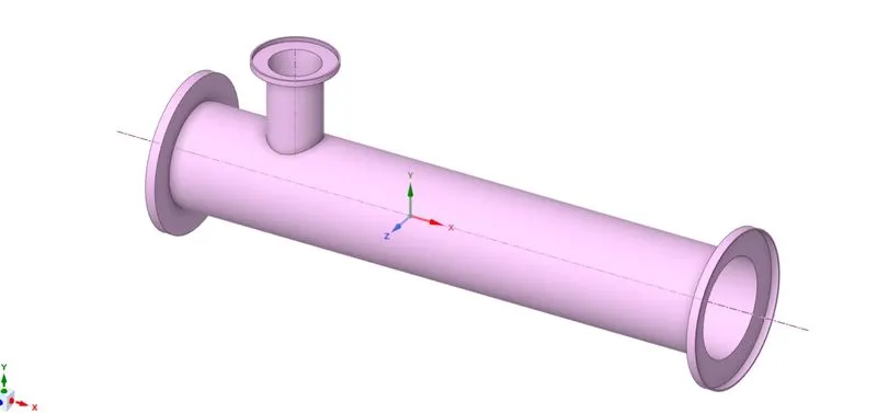
• Spaceclaim is a CAD cleanup and Pre-processing software module of ANSYS, used to prepare CAD geometries for further steps of simulation setup.
• CFD analysis requires a fluid volume, hence volume extract needs to be generated for the cavity where fluid will flow. Prepare -> Volume extract - > {select the edges at inlets and outlets} -> generate
• Once the fluid volume is generated, solid volume needs to be supressed and the fluid volume needs to be retained for further steps. This is because we are not interested in heat transfer analysis across the thickness of the pipe.

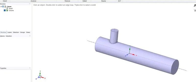
 Part 1 Step 2: Meshing

• The Fluid volume needs to be discretized by meshing the geometry. This can be done in the Ansys Mesher.
• Share the geometry with the geometry of ansys mesher module and open the mesher.
• Create Named selections: inlet_x, inlet_y, outlet_x, and wall.

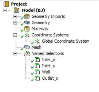
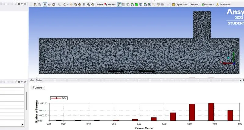
• Specify the mesh size and other parameters then generate the mesh.
• Check the mesh quality

Part 1 Step 3: Physics Setup and Solution

• This part of our study requires comparison between two different turbulence models. Hence two setups need to be created.
• One setup will be for k-omega turbulence model and the other for k-epsilon model.
• The geometry and mesh generated in previous steps will be shared between both setups.
• Double click on the “Setup” cell of the fluent module created for k-epsilon model.
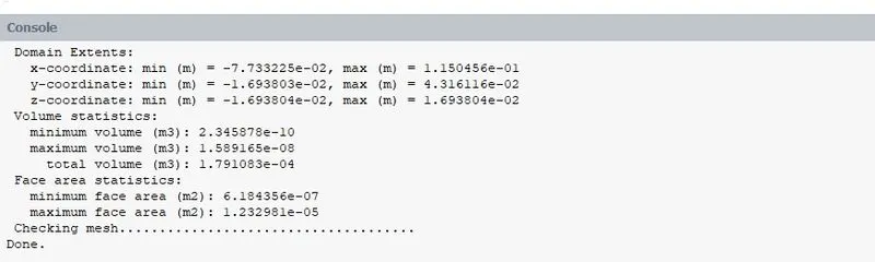
• “Domain” panel -> check mesh

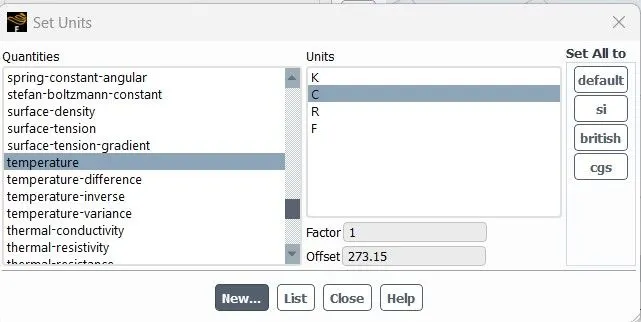
• “Domain” panel -> units -> change Temperature units from kelvin to C

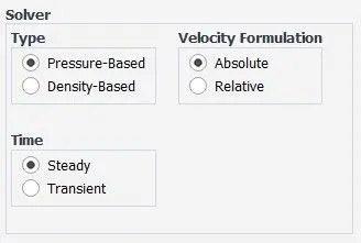
• Settings need to be specified for the physics of the domain. (Solver type -> pressure-based; velocity formulation -> Absolute; solver time -> steady)

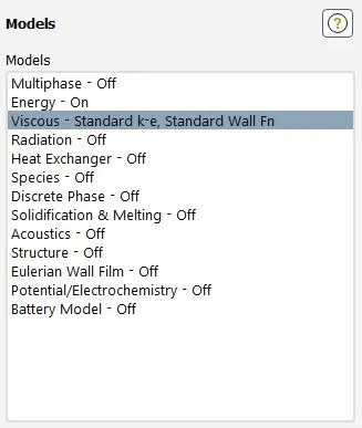
• Models -> Energy = on; Turbulence Model = k-epsilon (Accept the remaining default settings)

• In “Materials”, fluid material is air by default. Since our working fluid is also air we accept the default material.
• In the cell zone, material (air) is defined for the fluid volume.
• Boundary conditions
  • inlet_x -> velocity = 3 m/s, temperature = 36C
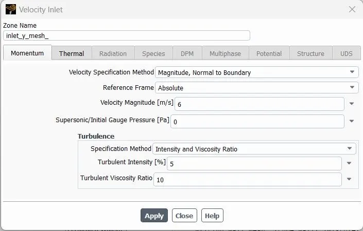
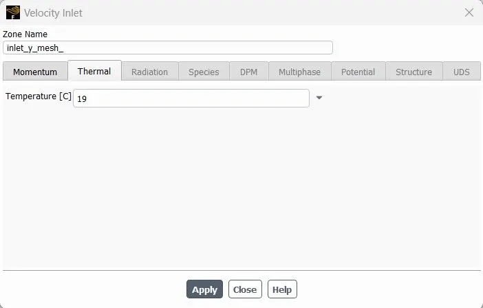
  • inlet_y -> velocity = 6 m/s (momentum ratio of 2), temperature = 19C
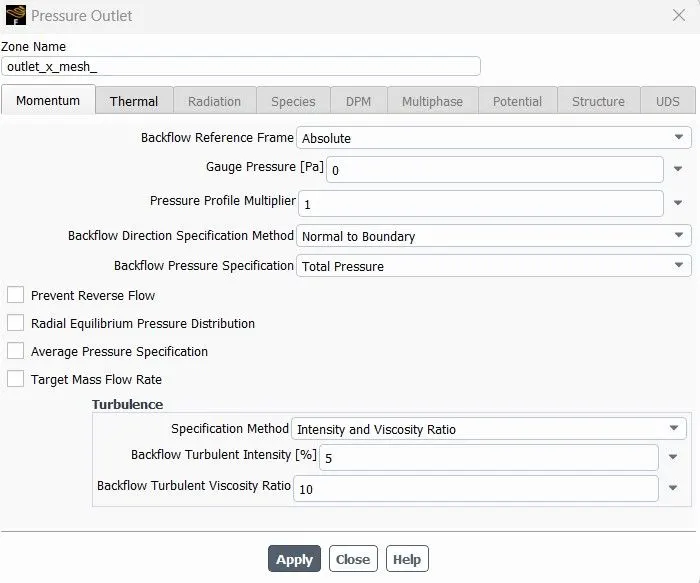
  • outlet_x -> pressure outlet (ambient pressure)

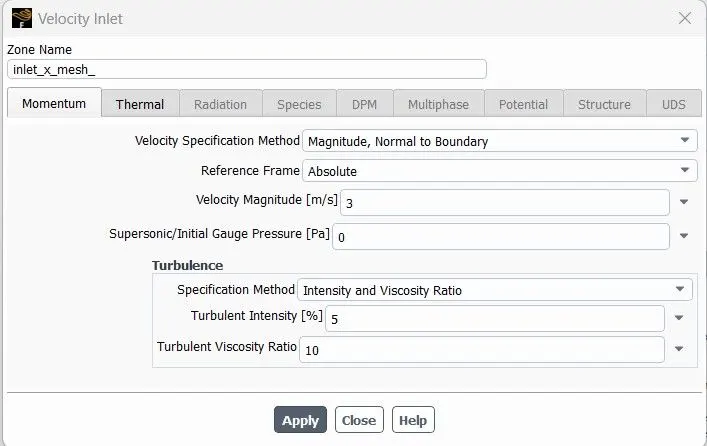
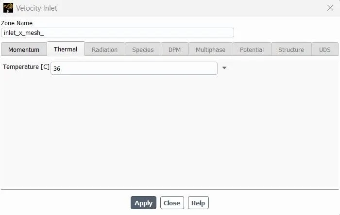
• Some solution monitors need to be created to evaluate the solutions.
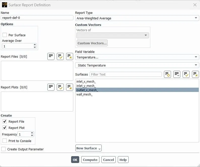
• Solution -> definitions -> surface report -> area-weighted average
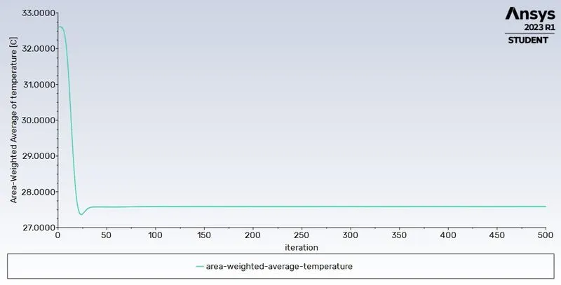
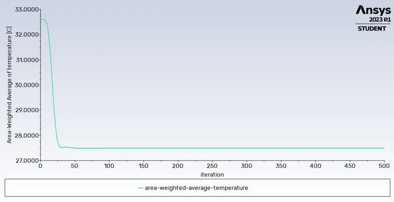
  • Monitor for area weighted average of temperature
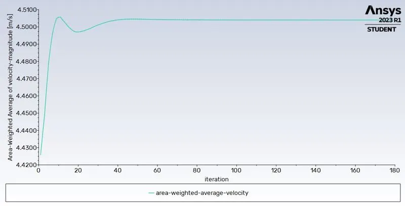
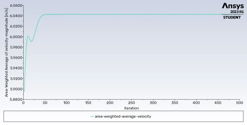
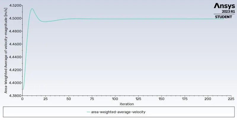
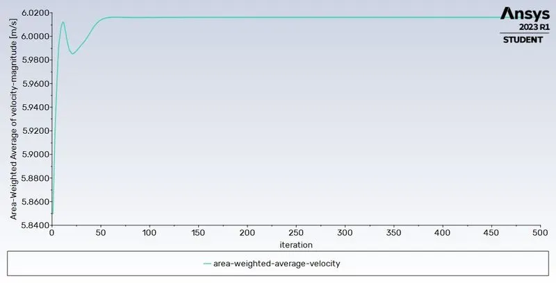
  • Monitor for area weighted average of velocity
• Solution -> definitions -> surface report -> Standard deviation
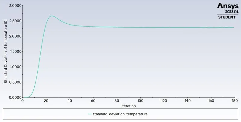
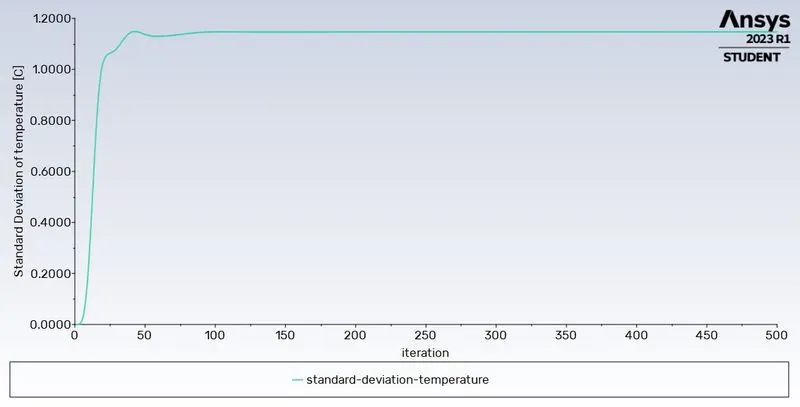
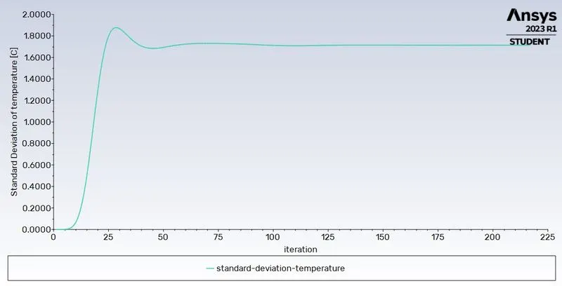
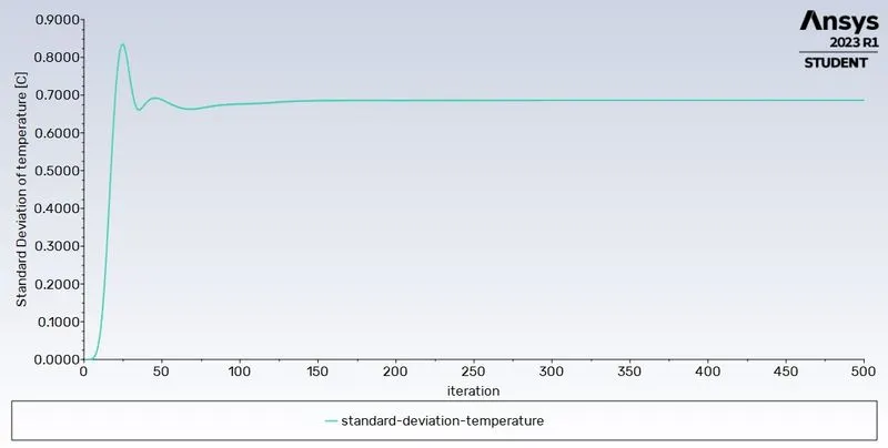
  • Monitor for Standard deviation of temperature
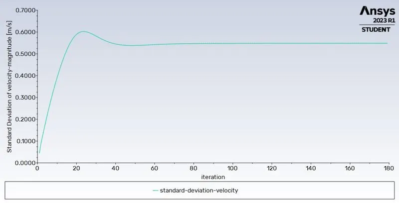
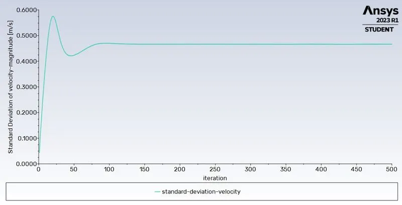
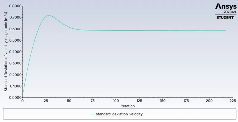
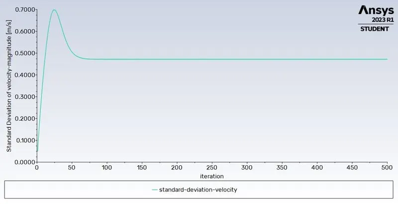
  • Monitor for Standard deviation of velocity

• Before starting the calculations, the solution needs to be initialized using hybrid initialization. Initialization creates an initial solution that the solver improves with each iteration

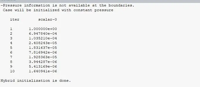
• After initializing the solution, the calculation can be started. “Start calculation” -> enter the number of iterations -> “calculate”
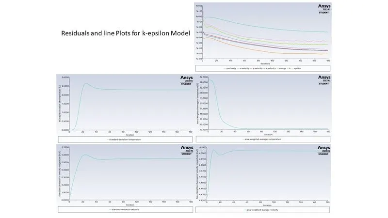
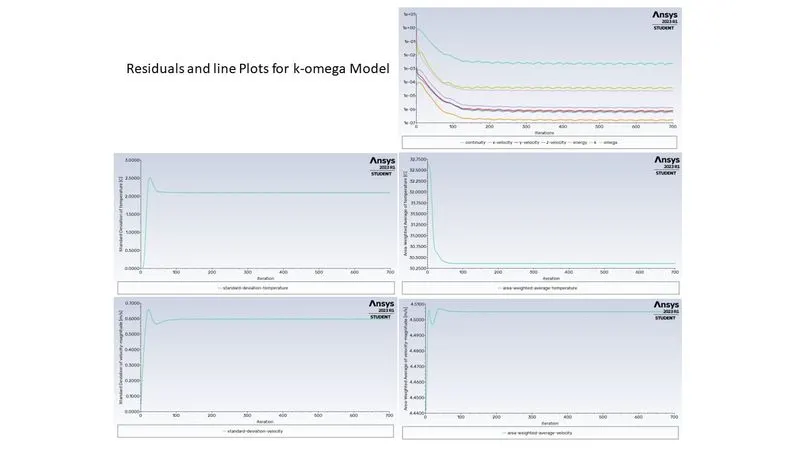
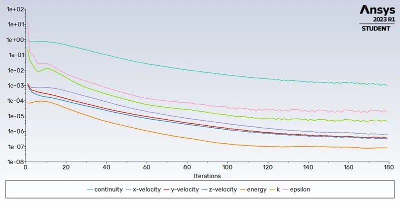
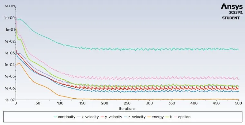
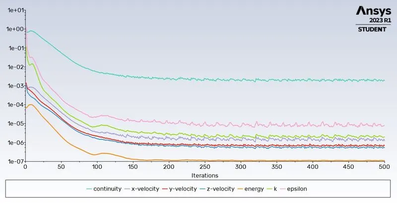
• Multiple plots are generated and updated as the iterations are done. These are: residuals, all monitors that we created earlier (area weighted average and standard deviation)
• Same process needs to be repeated for the k-omega turbulence model (this is why different setup files were created earlier)

Part 1 Step 4: Results

• After the calculations are done, ANSYS Fluent can be closed.
• The calculated results need to be processed further in “Post-processing”.
• Click on “Results” cell of ANSYS Fluent module in workbench. This will start up CFD-Post.
• To create a plane, Insert -> location -> plane. Then the parameters need to be specified based on the requirement.
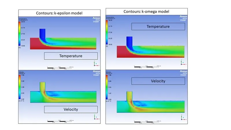
• These planes can be used to create contours by colouring them based n the respective variable.
• Contours created:
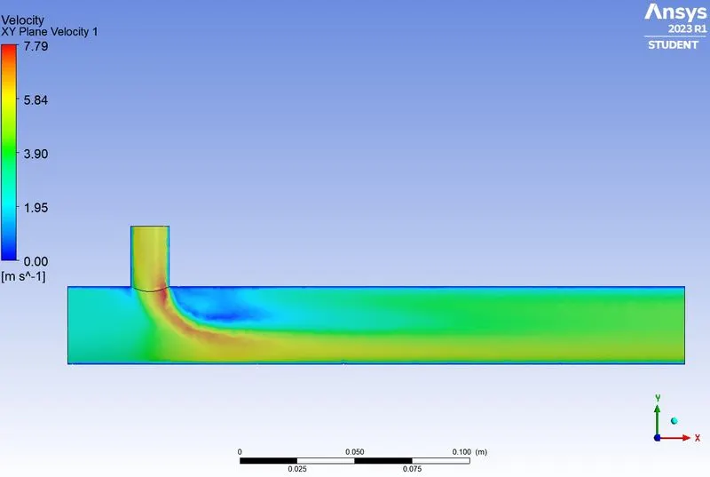
  • XY plane through centre (Temperature and Velocity)
• Above process needs to be done for both the setups.

Part 1 Step 5: observations

• Based on the results in part 1, it can be concluded that k-epsilon method is better suited since it gives a faster and better convergence of residuals.
• k-epsilon turbulence method also better captures the mixing of streams
• Also, the k-epsilon model predicts fluid flow more clearly for virtually far from the boundaries (wall), whereas the k-omega model predicts fluid flow more clearly near the wall. In our case, we are more interested in the phenomena occurring far from the walls.
• Therefore, k-epsilon turbulence method will be used for all subsequent calculations

Part 2: Mesh Independence Study

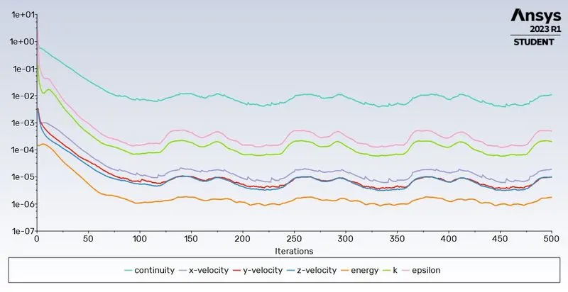
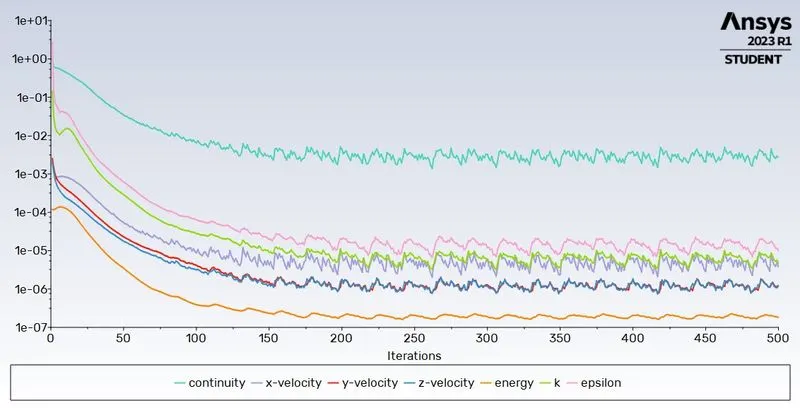
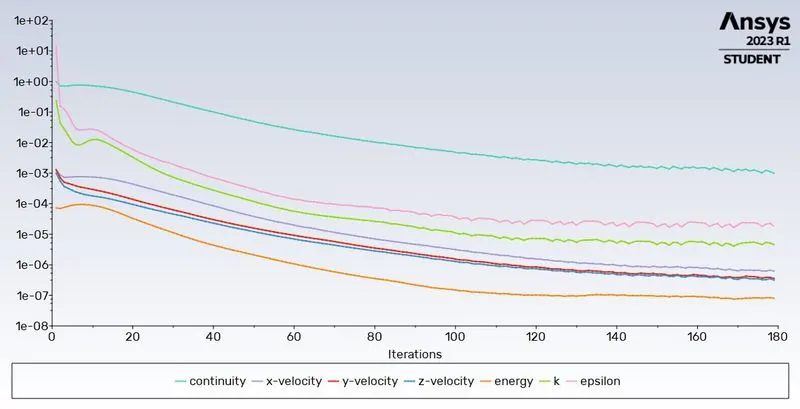
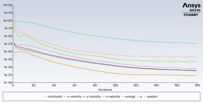
• Mesh Independence study needs to be performed to identify the best suited mesh parameters such that computational resources required are minimum and results obtained are sufficiently reliable.
• For this, starting with coarse mesh, mesh needs to be refined till the output of the value of interest becomes almost constant and/or a good convergence is attained.
• Analysis is performed for 4 different meshes as tabulated below.
• mesh size of 0.002 is selected without inflation layers, as it gives good convergence.

Mesh Size	Inflation Layer	Elements	Temperature - Outlet	Velocity - Outlet	Iteratiuons Specified	Iteratiuons run
			Celcius	[m s^-1]
0.01	None	12780	303.366	4.50813	500	500
0.005	None	22167	303.42	4.50087	500	500
0.002	None	106587	303.446	4.50328	500	179
0.002	Program Controled	106587	303.446	4.50328	500	179

Mesh Size 0.01

Mesh Size 0.005

Mesh Size 0.002

Mesh Size 0.002 with inflation layers

 Part 3: Simulation for mixing effectiveness

Part 3 Step 1: Setup

• The setup of main simulation cases is done in a manner same as described in part 1.
• Setups need to be created for each of the 4 cases under study (Case 1A, Case 1B, Case 2A, Case 2B)
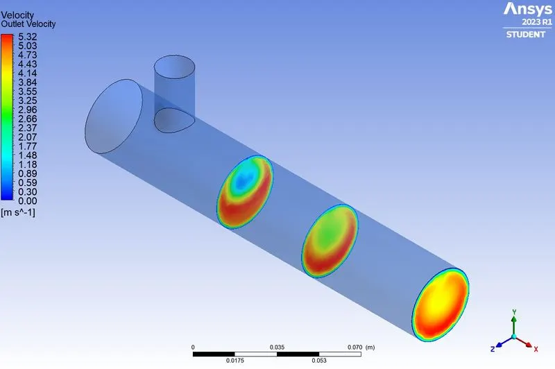
• Contours to be created for each of the 4 cases under study:
  • XY plane through centre (Temperature and Velocity)
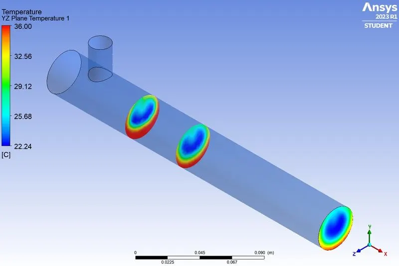
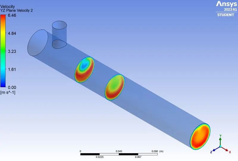
  • Contour at outlet (Temperature and Velocity)
  • YZ plane through centre (Temperature and Velocity)
  • YZ plane at x = 0.05 parameter (Temperature and Velocity)

Part 3 Step 2: Results

Case		Pipe length	Momentum Ratio	Specified Iterations	Cell count	Average outlet temperature	Number of iterations for convergence
1	A	Short	2	500	106587	30.3	179
1	B	Short	4	500	106587	27.59	calculation stopped at 500
2	A	Long	2	500	140990	30.39	217
2	B	Long	4	500	140990	27.49	calculation stopped at 500

Part 3 Step 3: Contours

Case 1 A

 

 

Case 1 B

 

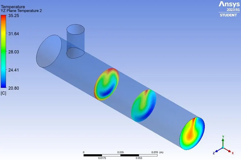
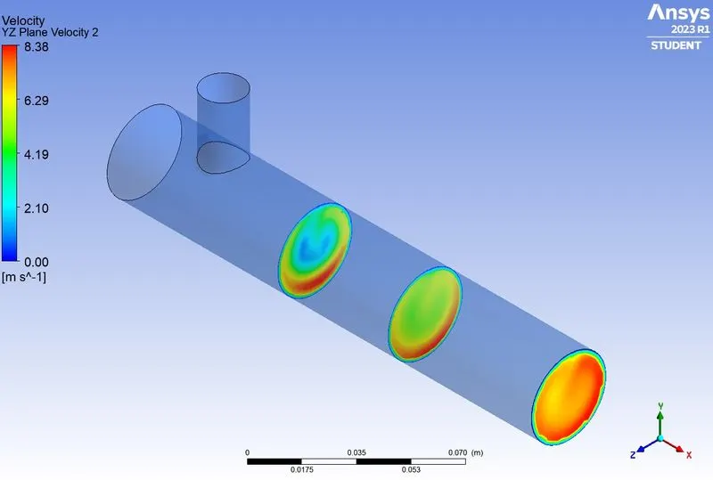
Case 2 A

 

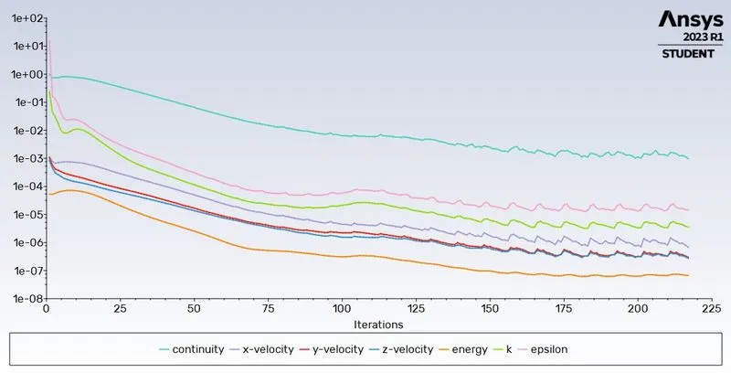
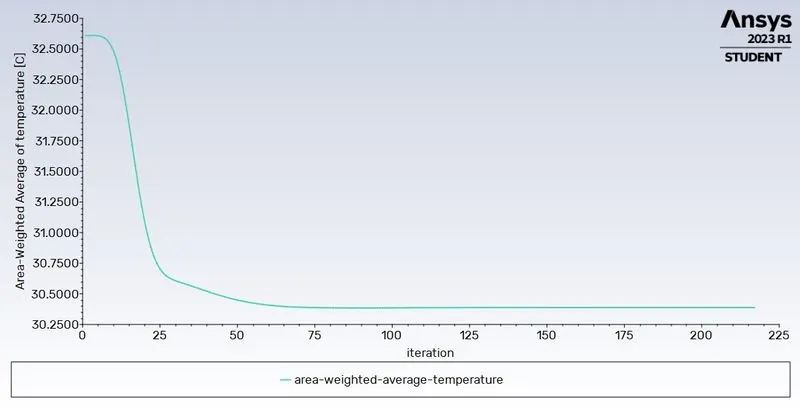
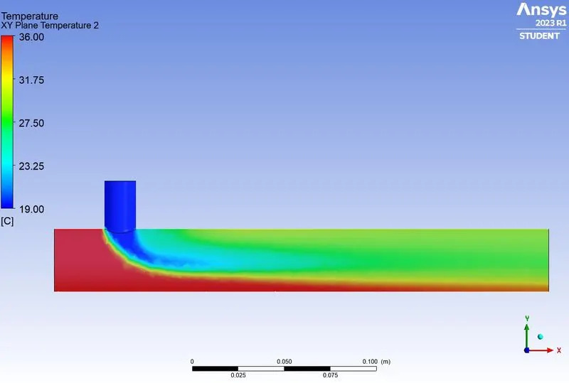
Case 2 B

 

 

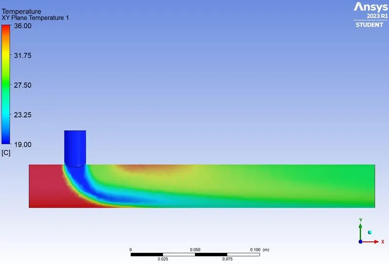
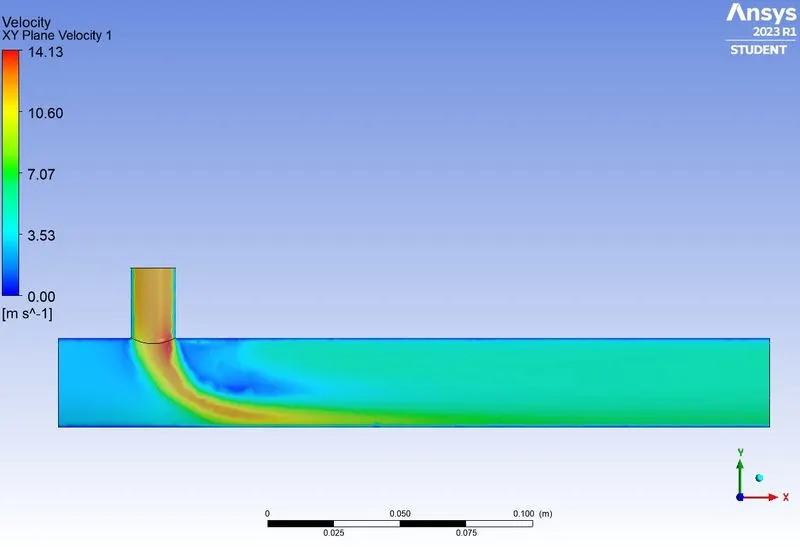
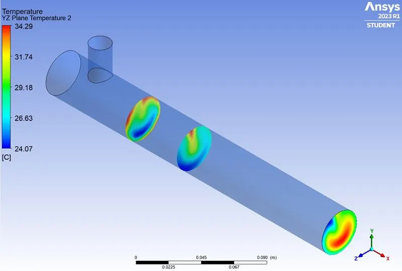
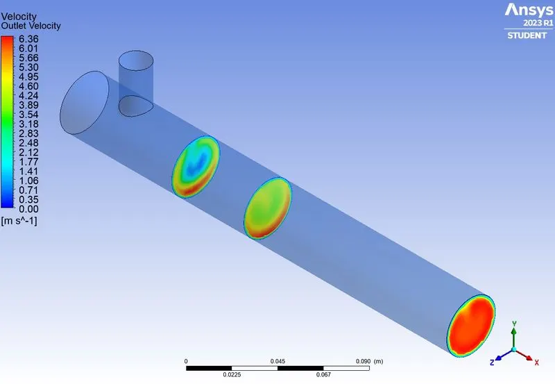
Results

Part1:

The k-epsilon turbulence model provides a better convergence of the solution residuals as compared to k-omega model for the current study.

Part2:

Mesh independence study indicates that a mesh size of 0.002 m is best suitable for the current study as it provides a better convergence of the solution residuals.

Part3:

Outlet Temperatures
Length	Momentum Ratio
	2	4
Short	30.3	27.59
Long	30.39	27.49

Conclusion

Part1:

The k-epsilon turbulence model is better suited for the current study as compared to k-omega model.

Part2:

Mesh size of 0.002 m is best suited for the current study.

Part3:

• Changing the Momentum ratio gives a better mixing of streams due to higher turbulence.
• Larger pipe length also increases mixing effectiveness due to diffusion but it is less compared to momentum ratio.
• Controlling the momentum ratio of hot and cold fluid streams is a more efficient way of mixing both the streams. Hence it provides better control over cooling.