Week 1- Mixing Tee

Aim: To perform steady-state simulation process of mixing of fluids inside a side-Tee, whith temperature difference. The impact of momentum ratio and length of the pipe is investigated in relation to effectiveness of mixing.

Introduction. We will be simulating mixing of hot and cold air inside a side-Tee setup using ANSYS FLUENT. The main aim is to estimate the effectiveness of mixing which is done by evaluating weighted average of temperature and also the standard deviation of temperature. We will first do a grid depandence test for the short Tee and then we will solve it using K-e and K- omega sst models of Turbulance. By comparing the two we select the better model for further simulation. Finally, we will investigate the flow and find the relation between mixing effectiveness and momentum ratio.

Case 1 :

Short mixing Tee with inlet velocity of hot fluid = 3 m/s.

Momentum ratio = 2,4

Case 2:

Long mixing Tee with inlet velocity of hot fluid = 3 m/s.

Momentum ratio = 2,4

Where,

Momentum ratio = Velocity of Cold fluid/Velocity of Hot fluid

Theorey:

Mixing in Tee:

A Tee is a configration allocated for mixing of fluids. It has numerous applications throughout industries. For example, the low viscosity or turbulant mixing is used in petrochemical industries for blending of some oils used as injection of additives and also blending of fuel gas.

Mixing Tee Configrations:

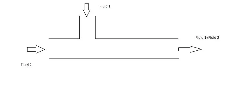
1. Side-Tee: Two pipes join at right angles to each other, one fluid stream enters straight through the main pipe and other enters perpendicularly.

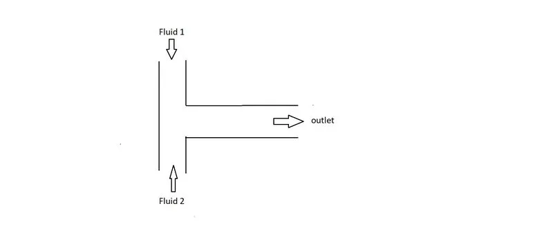
2. Opposed-Tee: Two opposing streams enters co-axially and leave through a pipe which is perpendicular to the entering streams.

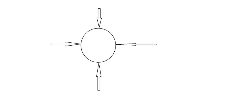
3. Mixed-Tee Mixer. Various fluid streams enters at a common place and the mixed outlet is vertically downwards.

Turbulant Mixing:

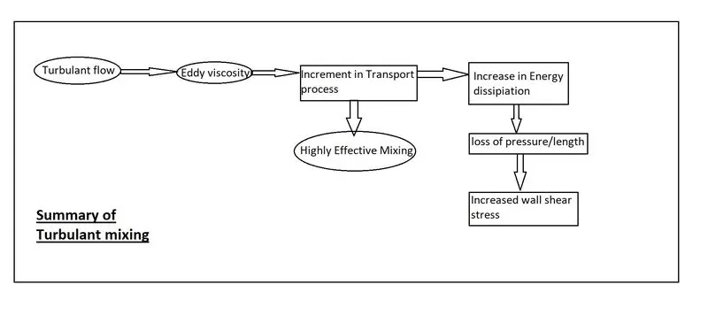
Turbulant flow is a flow, where fluid streams do not flow in an ordered uniform stremline flow, which is the case in laminar flow but instead flows in disorderd and random motion. The very characteristic of turbulant flow is the formation of spinning and swirling fluid structures called Eddies. These eddies are formed when there is a gradient of velocity in the flow. In the formation of these eddies, a significant part of mechanical energy of the fluid is utilised. These eddies produce fluctations in flow variables and they are eventually dissipiated as heat. In other words, formation and dissipiation of eddies is the reason turbulant flow is irreversible and incorporates entropy generation or loss of useful energy.

This brings the question, that if thermodynamically turbulant flow is inefficient, why is it used for mixing? The answer is that, the very presence of irreversibilities called eddies boost the process of mixing and mixing can be done more effectively in shorter length and in smaller time, at a small expence of increase in temperature due to entropy generation. The eddies interaact with each other as they move around, and they exchange momentum and energy. For example, the eddies near the center-line rotating with higher velocity, may move towards the wall and interact with eddies of smaller velocities. As they mix, momentum differences are smoothed out. Thus, in a way eddies in turbulant flow perform the job of viscosity in laminar flow, where due to molecular interactions momentum gradients are balanced. This way in turbulant flow we have eddy viscosity, since its magnitude is much greater than the molecular viscosity, Turbulant flows are more effective in mixing than laminar flows.

Moreover, the eddying motions can very quickly transport momentum, energy and heat from one place to another. As a result, gradients are smoothed out effectively, and the time averaged velocity profile in turbulant fow is much more uniform than in laminar flow.

Practical Significance of Turbulant Mixing where ΔT ≠ 0.

Mixing of fluids at a temperature gradient, leads to formation of hot and cold eddies which cause temperature fluctuations at the interface. This cause the temperature of adjoining wall surface to fluctuate. The induced thermal stresses on the walls keep on varying. This leads to a cyclic loading condition which is called Thermal stripping and causes a failure called thermal fatigue. If the freaquency of temperature fluctuations is in the range 0.1-10 Hz, thermal stripping is more likely to occur.

This makes study of turbulant mixing at temperature differance highly critical, since such procedures are carried out at Nuclear and other power plants, any component failure can result in catastrophic consequences.

Solving and Modelling Approach.

Mixing Tee Setup: We are having a side Tee where cold air is entering a varying velocity and is mixing with the hot air running horizantly.

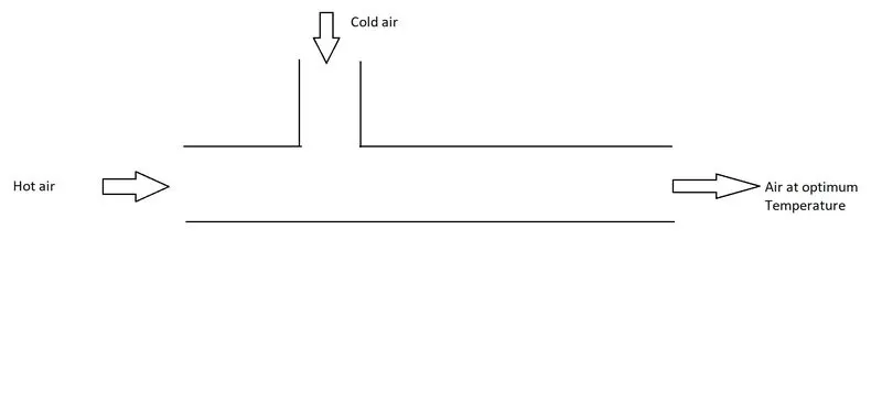
Estimation of Mixing Effectiveness-Strategy

We know that mixing will commence when the resulting mix of fluid reaches a Thermodynamic Equilibrium, that suggests the fluid will reach its Equilibrium Temperature which is supposed to be same everywhere. Thus, we can can measure the variation of Temperature at outlet we can measure for the level of mixing. To do this, we first calculate the weighted average of temperature at the outlet face and then we estimate the standard-deviation of temperature at that face, this will quantify the variation of temperature and we can estimate the mixing effectiveness.

Weighted average of temperature= Σ (Ti*Wi)/Σ Wi

Where,

Ti= Value of temperature at a discrete point on the outlet face.

Wi= weightage of Ti = the freaquency of occurance of that temperature at the face

Standard-deviation of Temperature = {Σ [(Ti-Tmean)/(n-1)]}^0.5

Where,

Ti= Value of temperature at a discrete point on the outlet face.

Tmean= Mean of temperature at the outlet face

n = number of observations

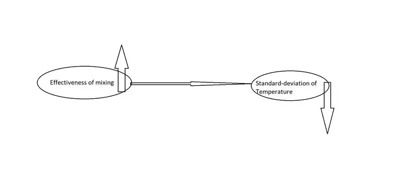
Case 1 :

Short mixing Tee with inlet velocity of hot fluid = 3 m/s.

Momentum ratio = 2,4

Steps Involved:

1. Setting up Workbench
2. Topological cleanup in ANSYS SPACECLAIM
3. Meshing with Unstructured Tetrahedral Elements
4. Setting up for solver in ANSYS FLUENT
5. Solving using k-𝛜 model for Turbulance and doing mesh dependancy test
6. As mesh lemgth is finalised, we run for k-Ω Turbulance model
7. Running the solution
8. Post processing in ANSYS CFD-POST
9. Following the same procedure for case 2.

Running the Grid Dependace Test for short pipe Momentum ratio = 4

1. Setting up ANSYS WORKBENCH

Topological cleanup in ANSYS SPACECLAIM

Here we extract the fluid volume and suppress the rest for simulation.

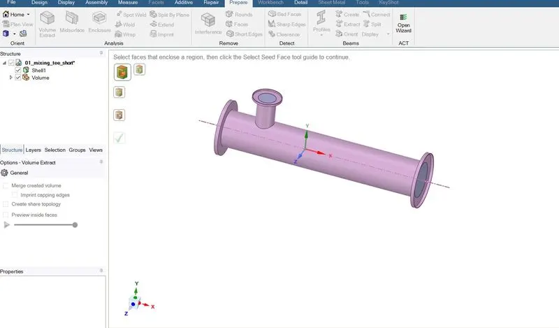
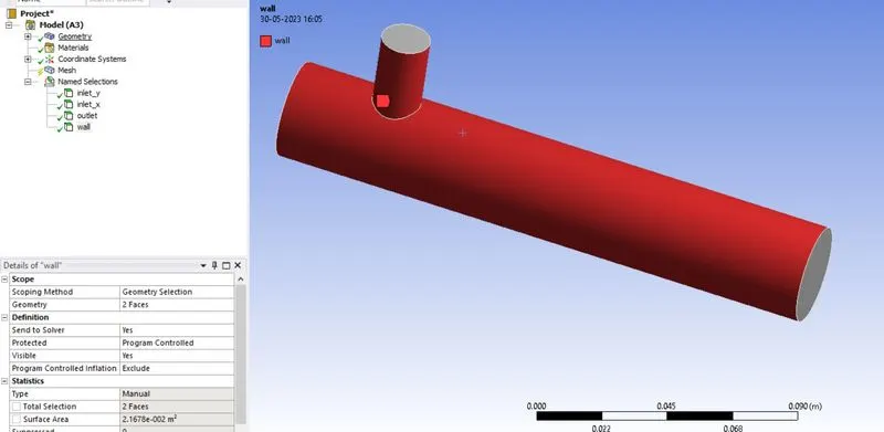
Setting up Boundires

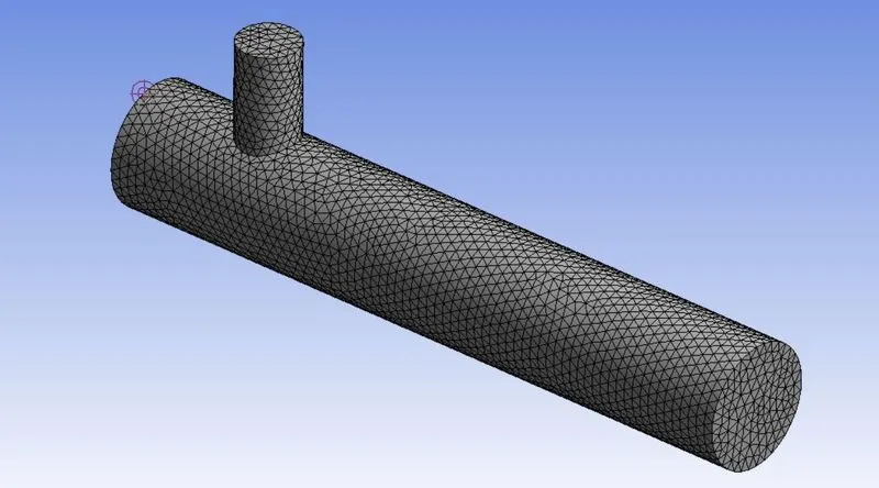
Meshing with Unstructured Tetrahedral Elements

We first mesh the model with default setup of ANSYS which is based upon the BONDING BOX.

Element size = 1.0219e-002 m ~ 10 mm

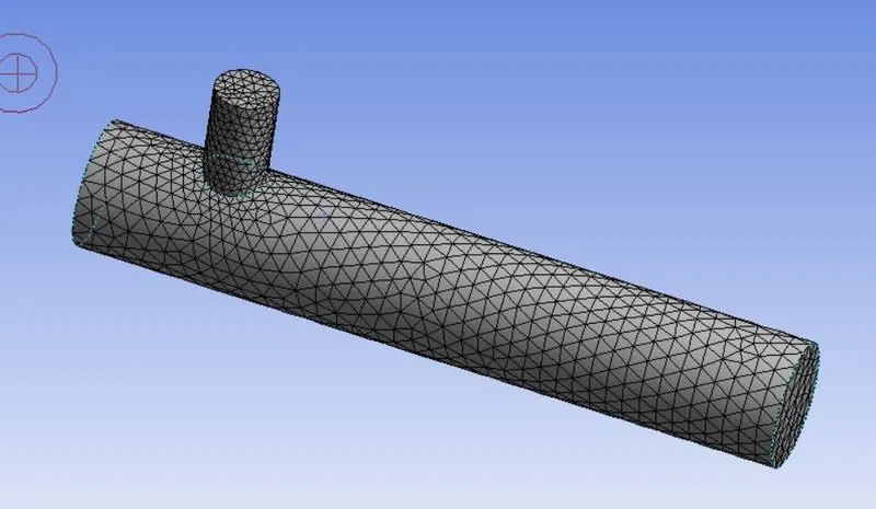
Checking for Mesh Quality

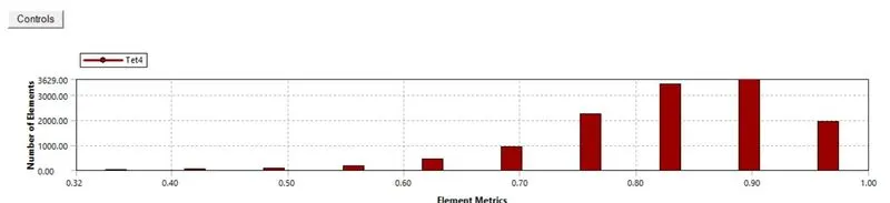
None of our elements are below 30% which is acceptable.

Setting up for solver

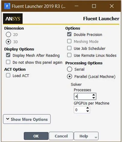
Solver

time= Steady-steady

Velocity formulation= Absolute

type= pressure based

Gravity= neglected

Energy Equation= Consdered for Temperature evaluation

Viscous Model = k-𝛜 2 equation, realizable with standard wall function

Material Specification:

Name = Air

Cp = Constant = 1006.43 J/kg

thermal conductivity k = 0.0242 w/m-k = constant

Although for real gases the heat capacity at cobstant pressure is not constant. For Ideal gases it is a function of temperature and is only constant for perfect gases. For air the variation of Cp with temperature is not very steep and for a smaller temperature range can be taken as constant. Taking Specific heat as constant is called Cold air standard assumption.

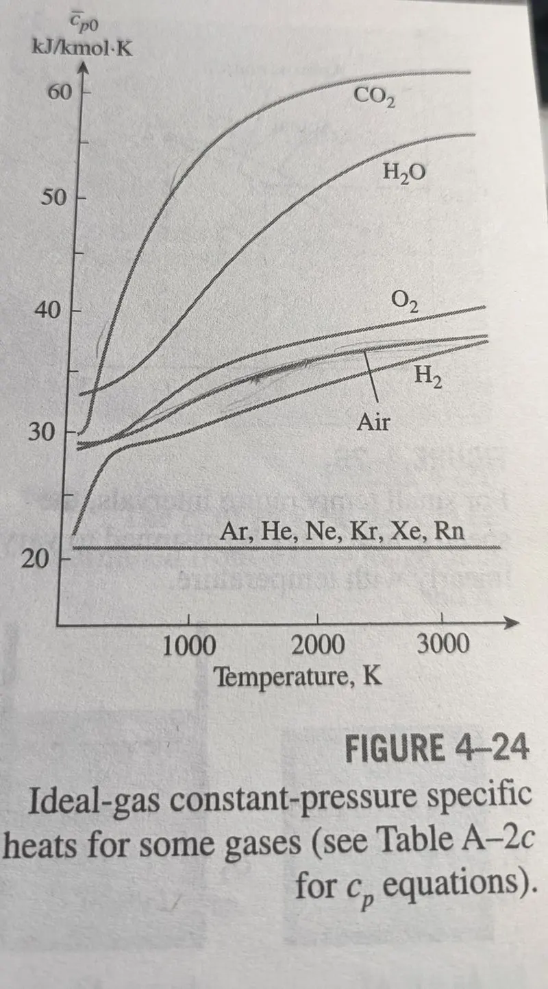
source= Thermodynamics by Y. A. CENGEL

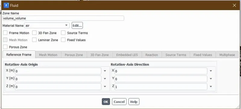
Setting up BOUNDRIES

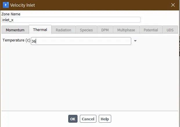
hot air inlet T=36 deg_C and V=3 m/s

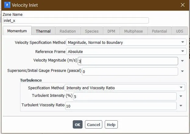
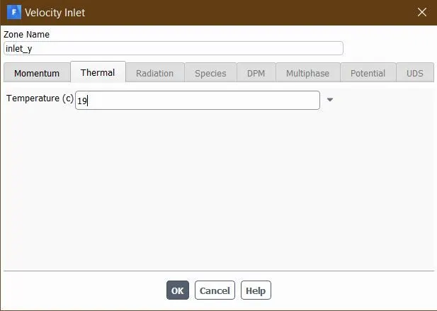
cold air inlet T=19 deg_C and V=12 m/s

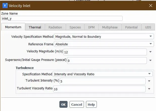
Outlet at atmospheric pressure so Pgauge = 0 bar

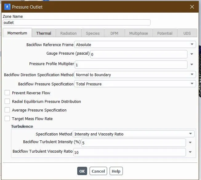
Setting up surface reports for outlet boundary

Area Weighted Average of Temperature

Standard Deviation of Temperature

Initialize the solution with Hybrid Initialization and then running the solution for 150 iterations to check for convergance

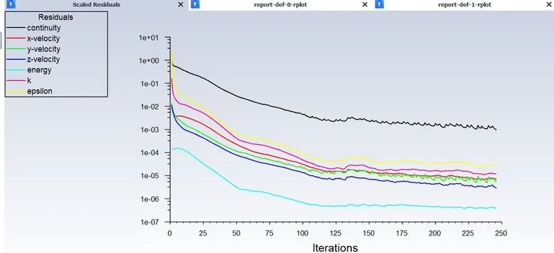
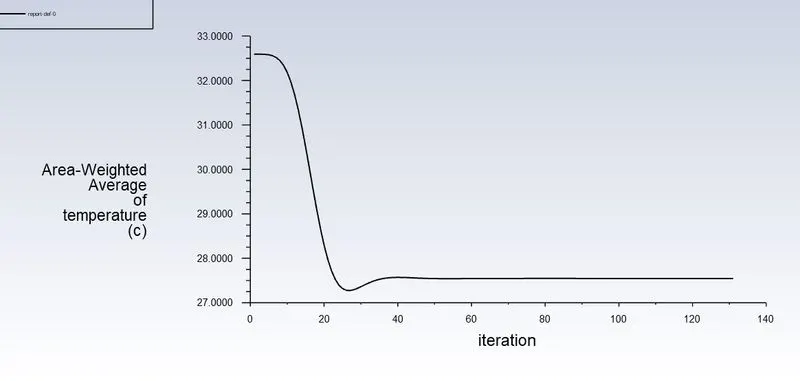
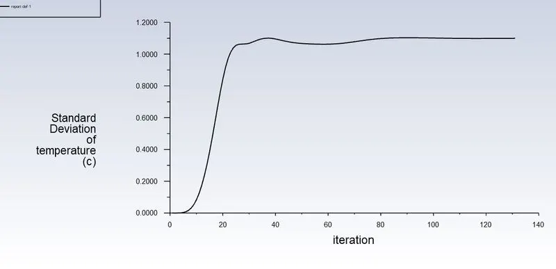
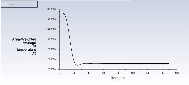
Solution Converged at 131 iteration with the following results

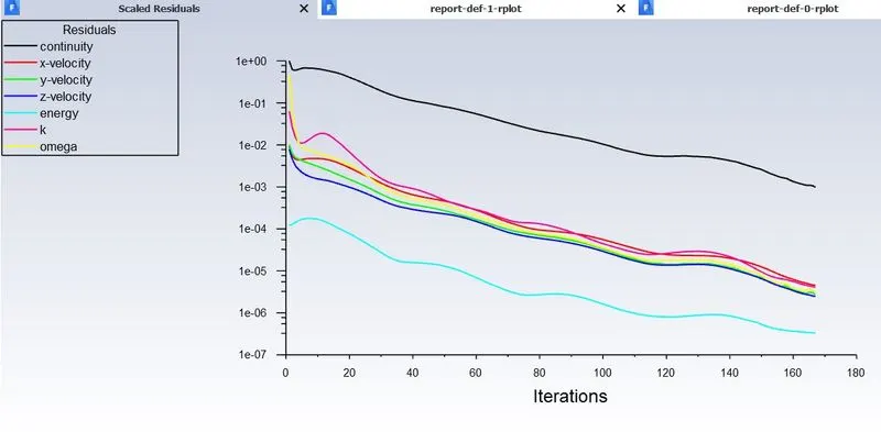
Residuals

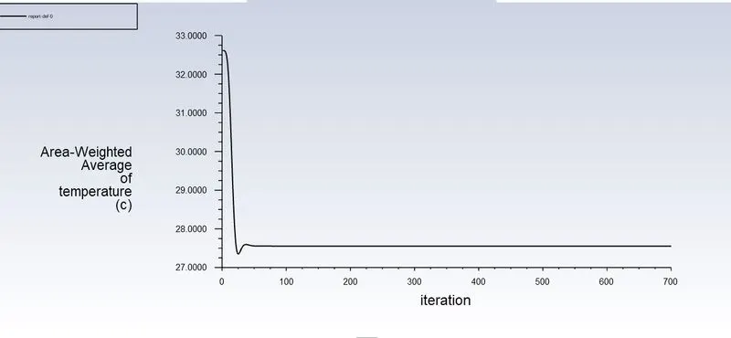
Area Weighted Average of Temperature

Standard Deviation of Temperature

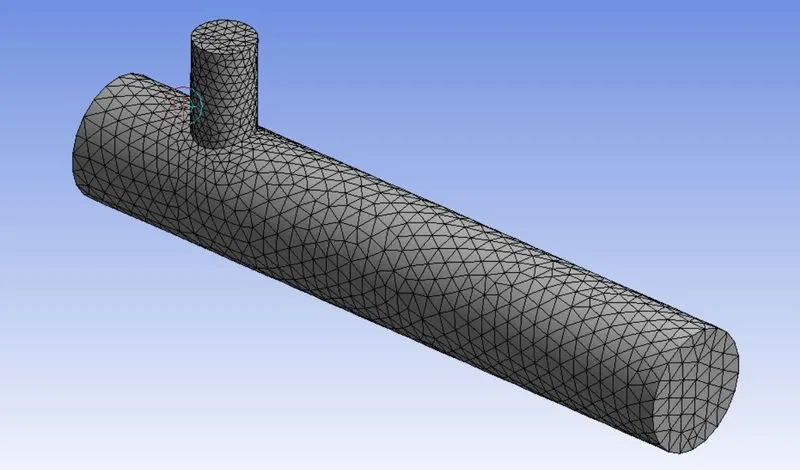
Reducing the Mesh Length to 5 mm

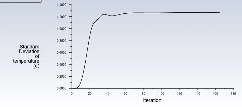
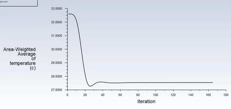
Running the solution

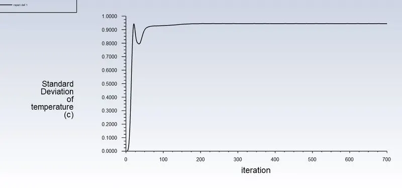
Standard Deviation of Temperature

Area Weighted Average of Temperature

Reducing the Mesh Length to 4 mm

Running the solution

Area Weighted Average of Temperature

Standard Deviation of Temperature

Reducing the Mesh Length to 3 mm

running the solution

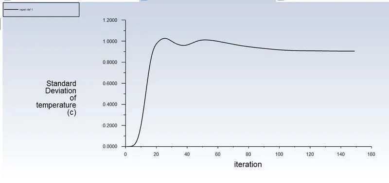
Standard Deviation of Temperature

Area Weighted Average of Temperature

Summary of Grid Dependance Test

Mesh Length (mm)	Number of Elements	Iterations taken for Solution Convergence	Weighted Average of Temperature (°C)	Standard-Deviation of Temperature
10	12760	131	27.5	1.25
5	14330	165	27.5	1.2
4	21977	Did not converge*	27.5	0.9
3	39790	149	27.5	0.9

*At mesh length of 4mm the continuity equation did not converge, however the rest of variables did converge.

Since, the only parameter changing in our grid dependance test is standard deviation of temperature, we select our mesh length on that basis.

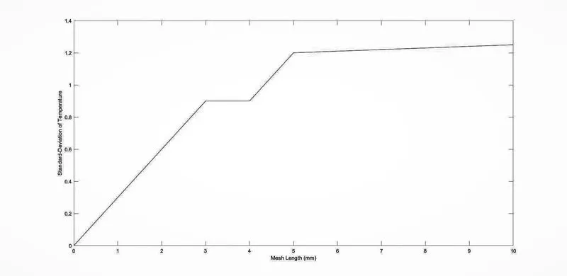
Result of Grid Dependance test=Mesh Length = 3mm

SETUP AND SOLVER:

CASE 1:

• Short mixing Tee with a hot inlet velocity of 3m/s
• Momentum ratio of 2,4

CASE 1.1:

• Short mixing Tee with a hot inlet velocity of 3m/s
• Momentum ratio of 2

SETUPS	SHORT TEE (MR=2 AND HOT INLET VELOCITY = 3m/s and cold inlet velocity = 6m/s)
	K-EPSILON	K-OMEGA
SOLVER TYPE	Pressure-based	Pressure-based
VELOCITY FORMULATION	Absolute	Absolute
TIME	Steady	Steady
VISCOUS MODEL	Realizable K-epsilon Model with standard wall function	K-omega SST model
MATERIAL	Air	Air
CELL ZONES	Fluid type : air	Fluid type : air
BOUNDARIES	· Inlet_x (velocity inlet) Velocity magnitude 3 m/s Temperature = 36 °C · Inlet_y (velocity inlet) Velocity magnitude = 6 m/s Temperature = 19°C · Outlet (pressure outlet) Gauge pressure = 0 pascal	· Inlet_x (velocity inlet) Velocity magnitude =3m/s Temperature = 36°C · Inlet_y (velocity inlet) Velocity magnitude =6m/s Temperature =19°C · Outlet (pressure outlet) Gauge pressure = 0 pascal

We set up mesh length = 3mm based upon our grid dependance test.

We follow the same steps to get the following results.

Results from K-e Model

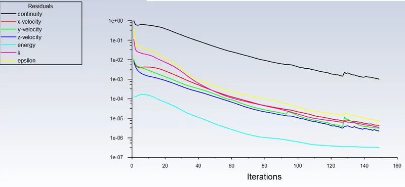
Residuals

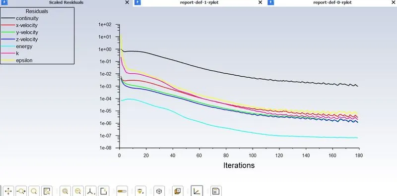
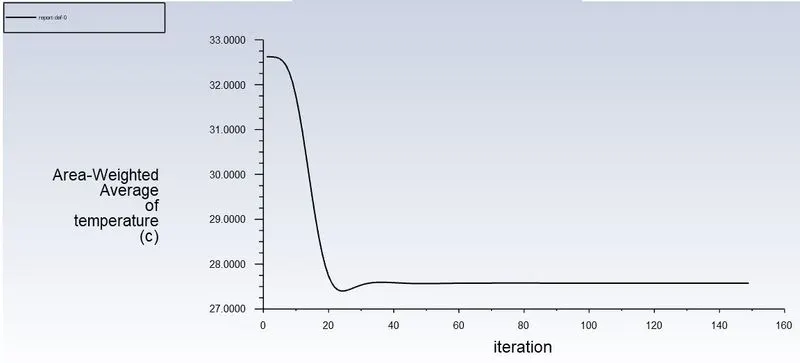
Weighted average of Temperature

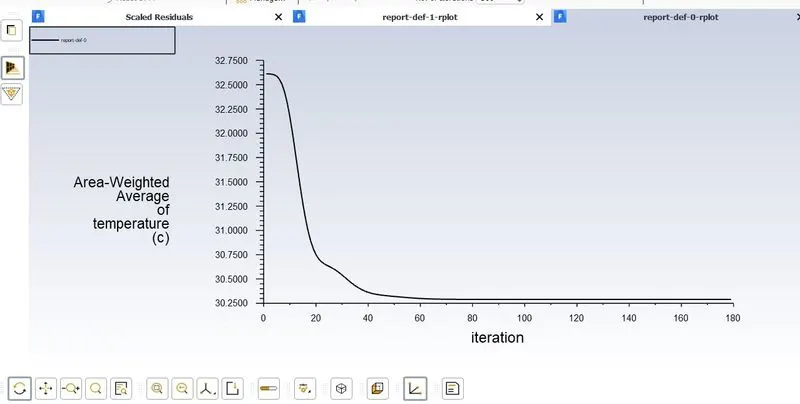
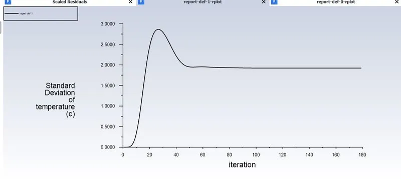
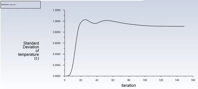
Standard Deviation of Temperature

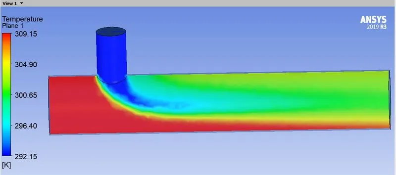
Temperature:

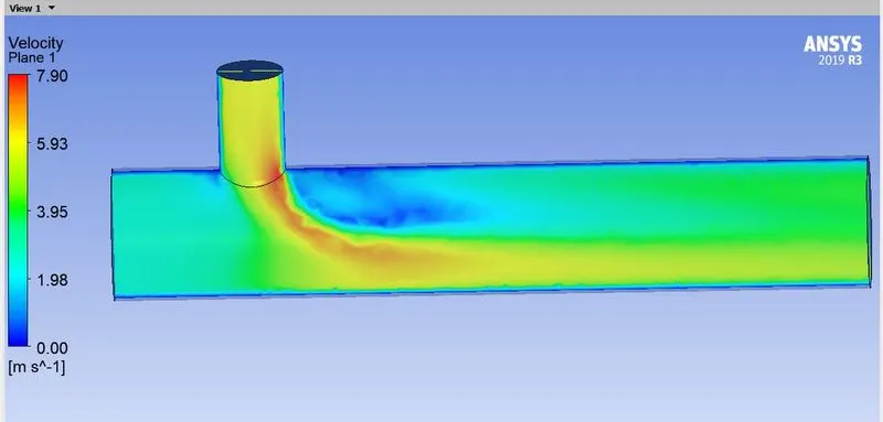
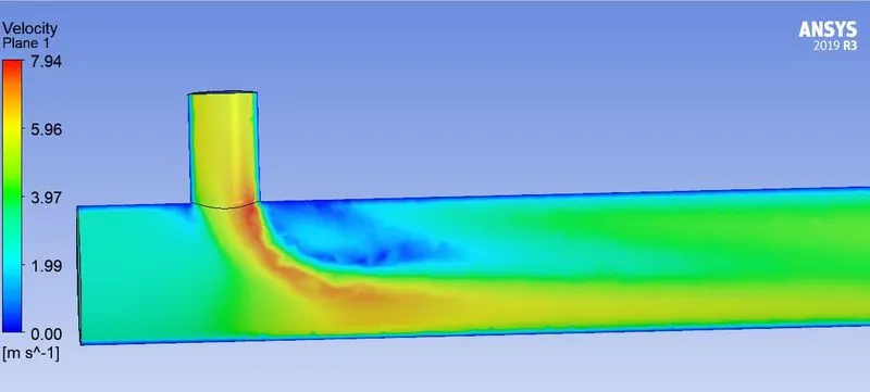
Velocity:

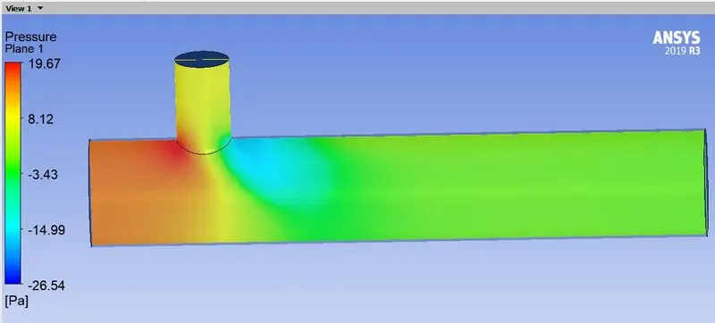
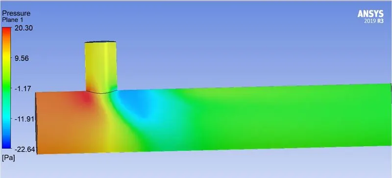
Pressure:

Results from K-Omega Model

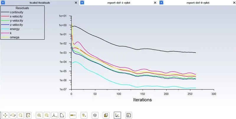
Residuals

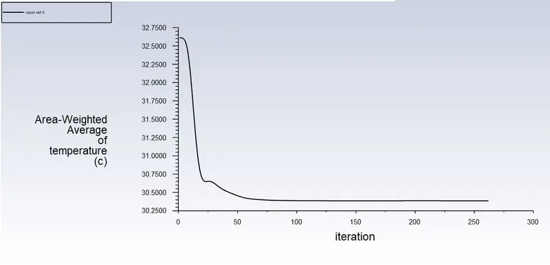
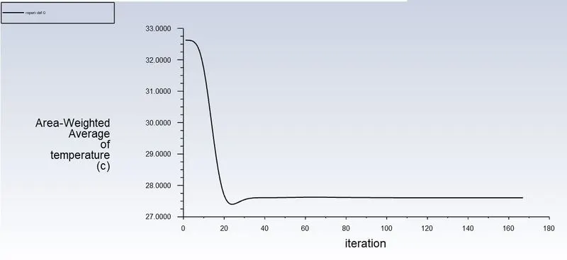
Weighted average of Temperature

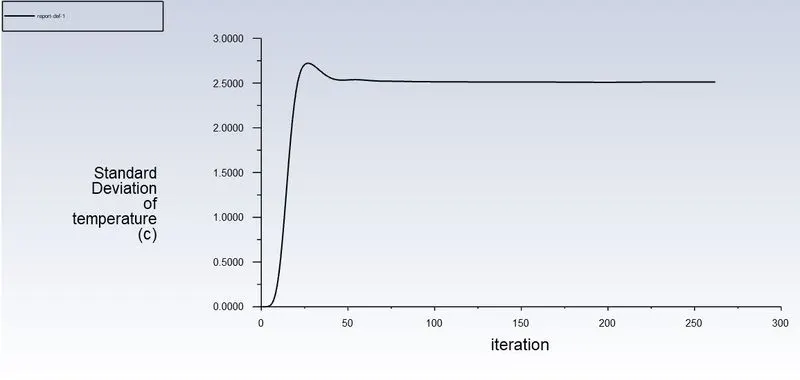
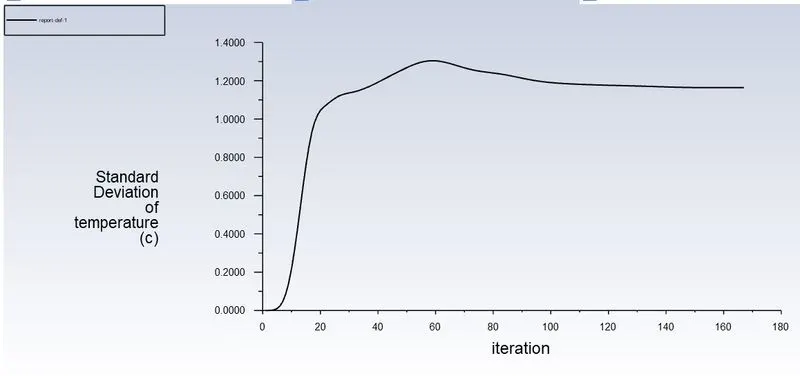
Standard Deviation of Temperature

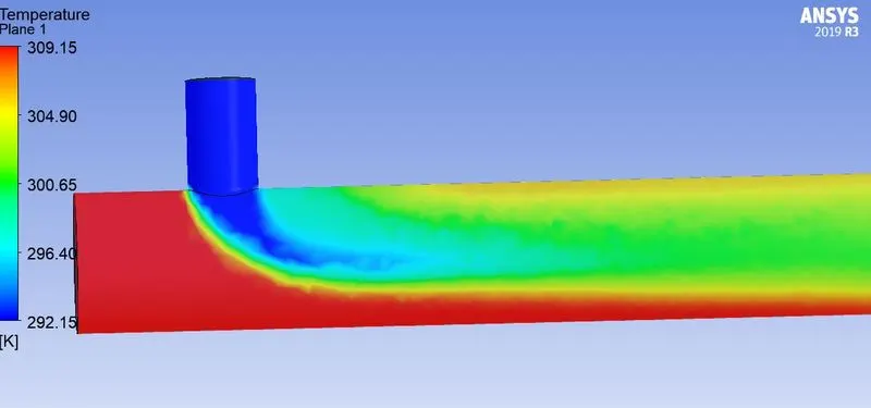
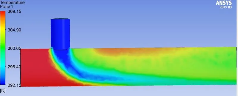
Temperature

Velocity

Pressure

Case 1.2

SETUPS	SHORT TEE (MR=4 AND HOT INLET VELOCITY = 3m/s and cold inlet velocity = 12m/s)
	K-EPSILON	K-OMEGA
SOLVER TYPE	Pressure-based	Pressure-based
VELOCITY FORMULATION	Absolute	Absolute
TIME	Steady	Steady
VISCOUS MODEL	Realizable K-epsilon Model with standard wall function	K-omega SST model
MATERIAL	Air	Air
CELL ZONES	Fluid type : air	Fluid type : air
BOUNDARIES	· Inlet_x (velocity inlet) Velocity magnitude 3 m/s Temperature = 36 °C · Inlet_y (velocity inlet) Velocity magnitude = 12 m/s Temperature = 19°C · Outlet (pressure outlet) Gauge pressure = 0 pascal	· Inlet_x (velocity inlet) Velocity magnitude =3m/s Temperature = 36°C · Inlet_y (velocity inlet) Velocity magnitude =12m/s Temperature =19°C · Outlet (pressure outlet) Gauge pressure = 0 pascal

Results for K-e Model

Reiduals

Weighted average of Temperature

Standard Deviation of Temperature

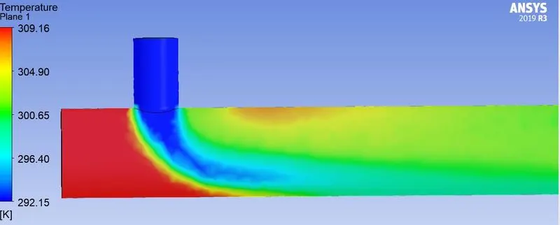
Temperature plot

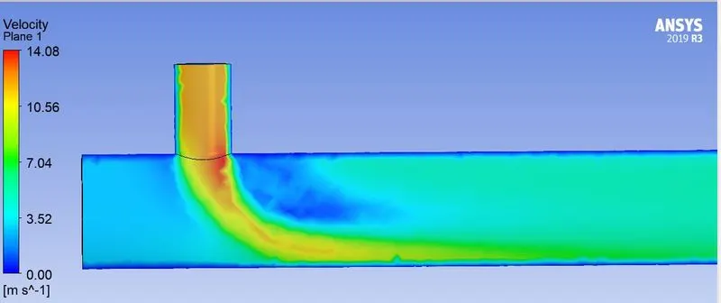
Velocity plot

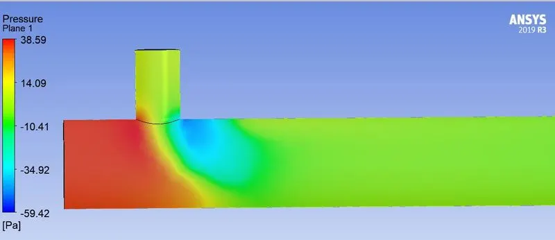
Pressure

Results for K-Omega Model

Residuals

Weighted average of Temperature

Standard Deviation of Temperature

Temperature Plot

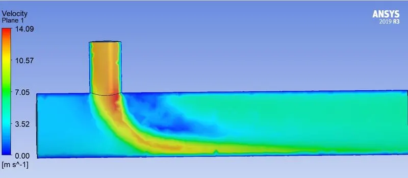
Velocity Plot

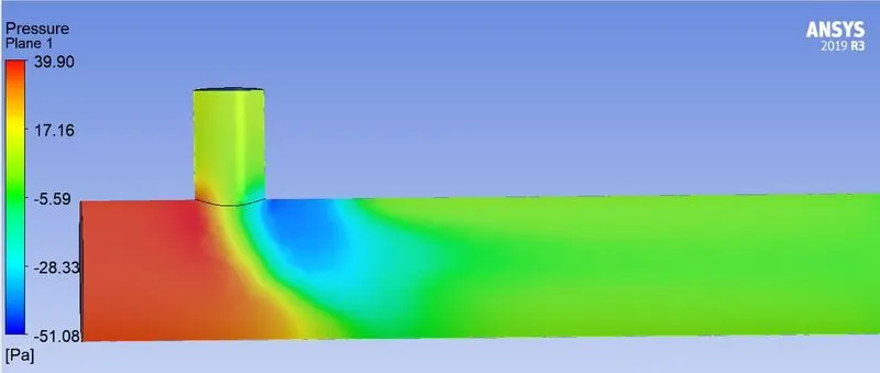
Pressure Plot

Comparing K-e and K-Omega Models for Case 1.1(Momentum ratio = 2)

Parameter	K-e	K-Omega-SST
Iterations	179	262
Std-deviation of Temperature	2.0	2.5
Weighted average of Temperature (°C)	30.25	30.35

Comparing K-e and K-Omega Models for Case 1.2(Momentum ratio = 4)

Parameter	K-e	K-Omega-SST
Iterations	149	167
Std-deviation of Temperature	0.9	1.1
Weighted average of Temperature (°C)	27.5	27.5

Comparing the results from K-e and K-Omega Models, we came to the following Conclusions

1. K-Omega-SST model requires more iterations to converge
2. Standard deviation of temperature for K-Omega-SST model is higher
3. Weighted average of temperature is nearly same for both models

Thus, we conclude that K-e 2 equation reliazable model of turbulance is performing better than K-Omega-SST model for this case. So, we will use K-e model for further study.

Case 2.1

SETUPS	SHORT TEE (MR=2 AND HOT INLET VELOCITY = 3m/s and cold inlet velocity = 6m/s)
	K-EPSILON
SOLVER TYPE	Pressure-based
VELOCITY FORMULATION	Absolute
TIME	Steady
VISCOUS MODEL	Realizable K-epsilon Model with standard wall function
MATERIAL	Air
CELL ZONES	Fluid type : air
BOUNDARIES	· Inlet_x (velocity inlet) Velocity magnitude 3 m/s Temperature = 36 °C · Inlet_y (velocity inlet) Velocity magnitude = 6 m/s Temperature = 19°C · Outlet (pressure outlet) Gauge pressure = 0 pascal

Results

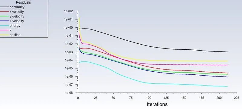
Residuals

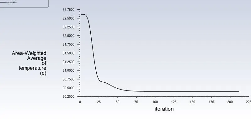
Weighted average of Temperature

Standard Deviation of Temperature

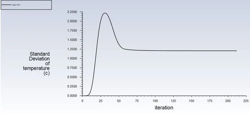
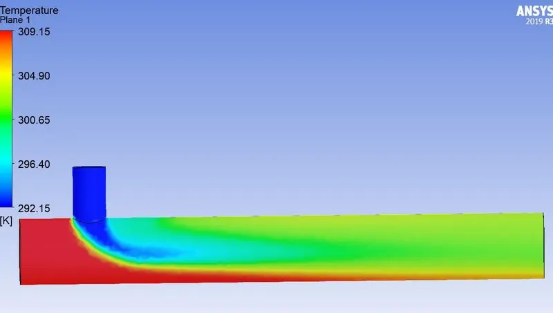
Temperature Plot

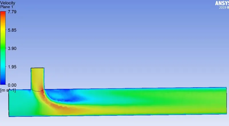
Velocity

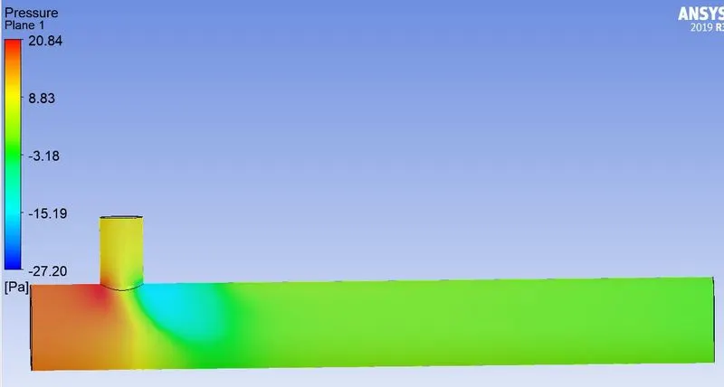
Pressure

Case 2.2

SETUPS	SHORT TEE (MR=4 AND HOT INLET VELOCITY = 3m/s and cold inlet velocity = 12m/s)
	K-EPSILON
SOLVER TYPE	Pressure-based
VELOCITY FORMULATION	Absolute
TIME	Steady
VISCOUS MODEL	Realizable K-epsilon Model with standard wall function
MATERIAL	Air
CELL ZONES	Fluid type : air
BOUNDARIES	· Inlet_x (velocity inlet) Velocity magnitude 3 m/s Temperature = 36 °C · Inlet_y (velocity inlet) Velocity magnitude = 12 m/s Temperature = 19°C · Outlet (pressure outlet) Gauge pressure = 0 pascal

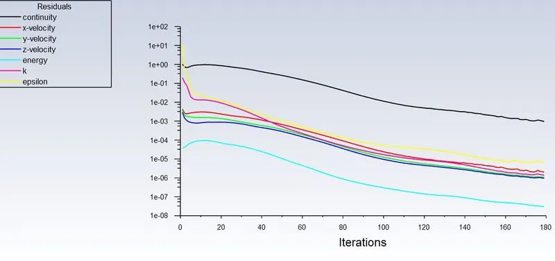
Residuals

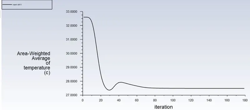
Weighted average of Temperature

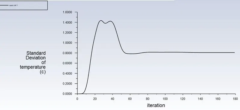
Standard Deviation of Temperature

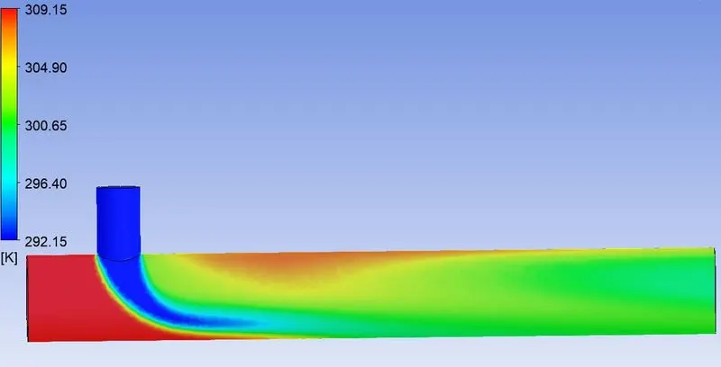
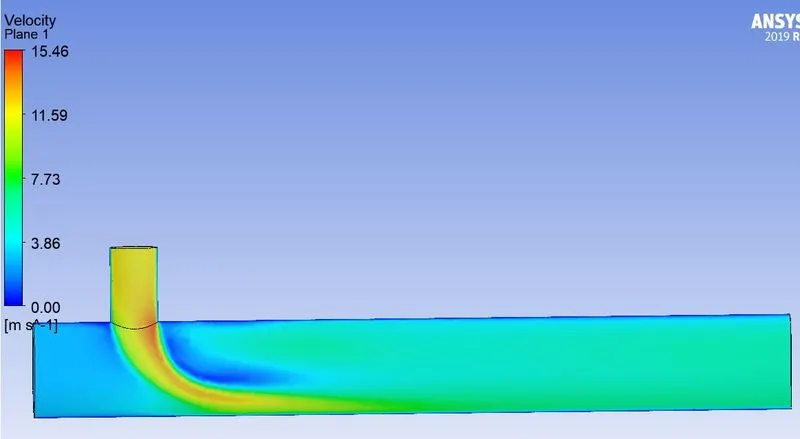
Temperature Plot

Velocity

Pressure

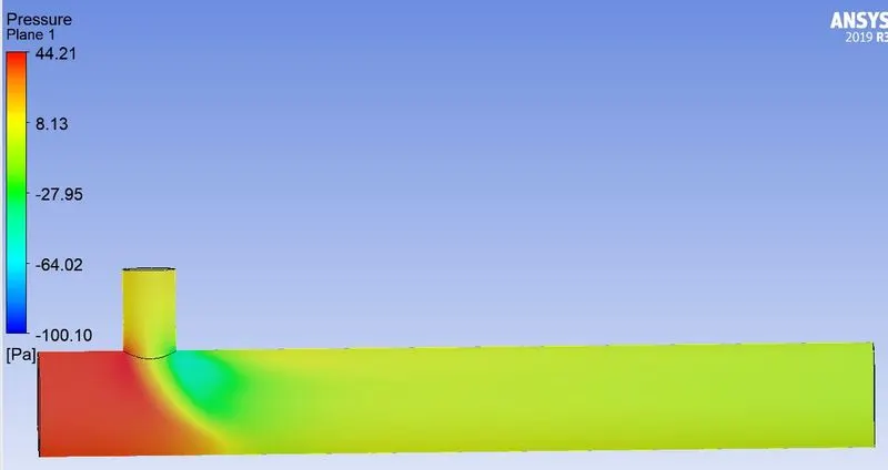
Summarising Data from all Cases

Parameter	Short Tee (M=2)	Long-Tee (M=2)	Short Tee (M=4)	Long-Tee (M=4)
Cell Count	39790	140510	39790	761482
Iterations for Convergance	179	212	149	179
Weighted Average of Temperature (°C)	30.25	30.35	27.5	27.5
Standard-Deviation of Temperature	2.0	1.25	0.9	0.8

Where M=momentum ratio

Observations:

1. It is clear that the weighted average of temperature at the outlet is depending on momentum ratio and not on the length of the pipe.
2. The Cell count increased considerably with longer pipe which has no considerable effect on mixing. Thus using longer pipe is unnecessary burden on computational resources.
3. Number of iterations for convergance increased with increasing momentum ratio, as flow becomes more turbulant more discrepencies are there to handle.

Conclusion:

The mixing effectiveness = f(momentum ration). Thus for effective mixing we should use a higher momentum ratio with a pipe of shorter length.

Analytical Calculations

Considering the system to follow an internally reversible process, the outlet temperature can be calculated as;

Consider it Euation 1

Where,

Tmixture = Temperature at outlet

T_hot = Temperature of Hot air (K)

T_cold = Temperature of cold air (K)

m_hot= mass flow rate of hot air (kg/s)

m_cold= mass flow rate of cold air (kg/s)

Now,

Mass flow rate = Density*Area*Velocity

A1=Area of hot air inlet (m*m)

A2=Area of cold inlet (m*m)

V1=Velocity of hot air (m/s)

V2=Velocity of cold air (m/s)

Therefore,

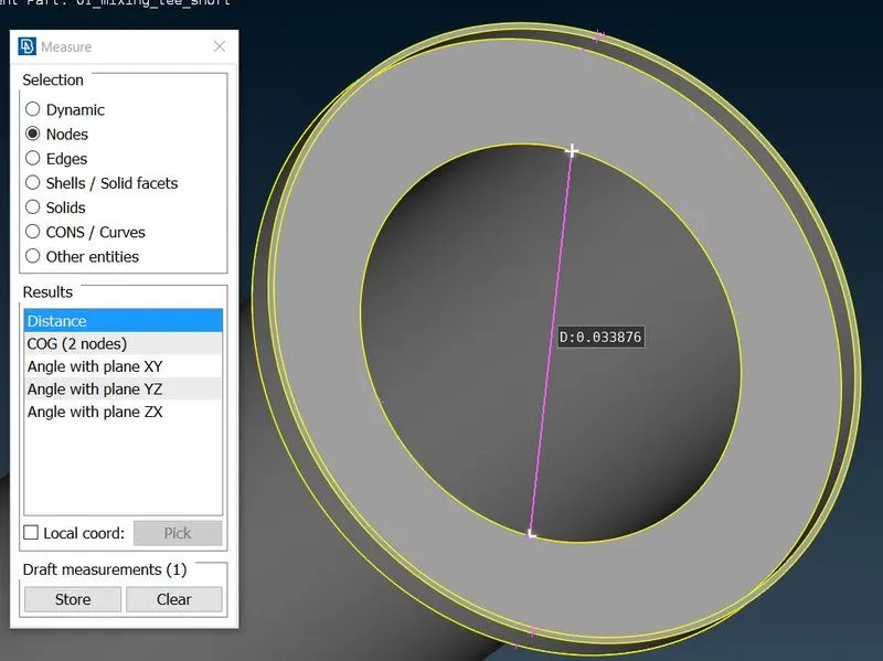
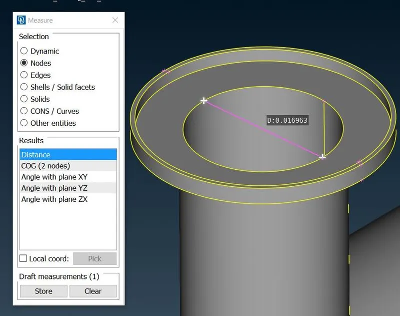
We estimated the required areas by measuring diameter using Measure tool of ANSA

D_hot_inlet=D1=0.33876m

D_cold_inlet=D2=0.01693m

Thus,

A1=pi/4*D1^2=8.09069e-4

A2=pi/4*D2^2=2.2527e-4

For M=2

V1=3m/s

V2=6m/s

For M=4

V1=3m/s

V2=12m/s

For M=2

m_hot=ρ_air*A1*V1=3.2733e-3 (kg/s)

m_cold=ρ_air*A2*V2=1.655e-3 (kg/s)
T_hot=309 (K)

T_cold=292 (K)

Using Equation 1

T_mixture=[3.2733e-3 (kg/s)*309 (K)+1.655e-3 (kg/s)*292 (K)]/(3.2733e-3 (kg/s)+1.655e-3 (kg/s)) = 303.599 K = 30.66 °C; from our results T_mix=30.25 °C

Similarly, for M=4

m_hot=ρ_air*A1*V1*4=3.2733e-3 (kg/s)

m_cold=ρ_air*A2*V2*4=3.3092e-3 (kg/s)

T_mixture=[3.2733e-3 (kg/s)*309 (K)+3.3092e-3 (kg/s)*292 (K)]/(3.2733e-3 (kg/s)+3.3092e-3 (kg/s)) = 300.454 K = 27.45 °C; from our results T_mix=27.5 °C

This validates our Simulation.