Week 1- Mixing Tee
AIM
- To do steady state simulation of mixing of two fluids in a mixing tee with 36 degree celsius and and 19 degree celsius as the inlet temperatures.
- To find out the mixing effectiveness in two cases, a short mixing tee and a long mixing tee.
- Use K-epsilon and k-omega model for the simulations and find out which model is best suitable for the simulation.
- To plot velocity and temperature contours in the cut section plane of the model.
- To find out the dependency of length and momentum ratio in effectiveness of the mixing.
- Tabulate the results.
INTRODUCTION AND THEORY
Mixing tee is widely used all around the world to mix two fluid mediums generally at two different temperatures and velocity to control the outlet temperature. The geometry is specifically designied to facilitatae effective mixing of the fluids. Inlet velocities of the fluid, Inlet temperatures and mixing length of the Tee are major factors which control the mixing of the fluids. We can vary these factors to control the mixing of the fluids. Mixing Tees are widely used for blending, agitation, recirculation, mixing, aeration and heating.
K-epsilon model
The k-epsilon (k−ϵ) model is commonly used to simulate the mean flow characteristics for turbulent flow conditions. It belongs to the Reynolds-averaged Navier Stokes (RANS) family of turbulence models where all the effects of turbulence are modeled.
It is a two-equation model. That means that in addition to the conservation equations, it solves two transport equations (PDEs), which account for effects like convection and diffusion of turbulent energy. The two transported variables are turbulent kinetic energy (k), which determines the energy in turbulence, and turbulent dissipation rate (ϵ), which determines the rate of dissipation of turbulent kinetic energy.
The k−ϵ model is shown to be reliable for free-shear flows, such as the ones with relatively small pressure gradients, but might not be the best model for problems involving adverse pressure gradients, large separations, and complex flows with strong curvatures.
K-omega model
The k-omega (k−ω) turbulence model is one of the most commonly used models to capture the effect of turbulent flow conditions. It belongs to the Reynolds-averaged Navier-Stokes (RANS) family of turbulence models where all the effects of turbulence are modeled.
It is a two-equation model. That means in addition to the conservation equations, it solves two transport equations (PDEs), which account for the effects like convection and diffusion of turbulent energy. The two transported variables are turbulent kinetic energy (k), which determines the energy in turbulence, and specific turbulent dissipation rate (ω), which determines the rate of dissipation per unit turbulent kinetic energy. ω is also referred to as the scale of turbulence.
The standard k−ω model is a low Re model, it can be used for flows with low Reynolds number where the boundary layer is relatively thick and the viscous sublayer can be resolved.
Thus, the standard k−ω model is best used for near-wall treatment. Other advantages include a superior performance for complex boundary layer flows under adverse pressure gradients and separations (e.g., external aerodynamics and turbomachinery). On the contrary, this model has also shown to predict excessive and early separations.
Procedure
- Our first task is to import the geometry into spaceclaim to extract the fluid volume.
- Open Fluent workbench. Double click on geometry to open spaceclaim.
- Import the geometry by File>Open>file location.
- Once the file is opened we can extract the fluid volume.
- Go to prepare module and click extract volume.
- Select the edges of the two inlet and outlet using the edge selection option and click the green tick. The volume is generated.
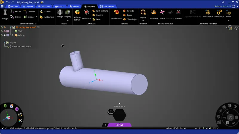
- Once the volume is extracted, we can exclude the body from simulation since we are concerned about the fluid flow happening inside the geometry.
- Right click on shell>select exclude from simulation. The body is now excluded from simulation.
- Next we can move onto the meshing process.
- Double click on the mesh in fluent workbench.
- Once the geometry is opened in the mesh module, we can create named selection.
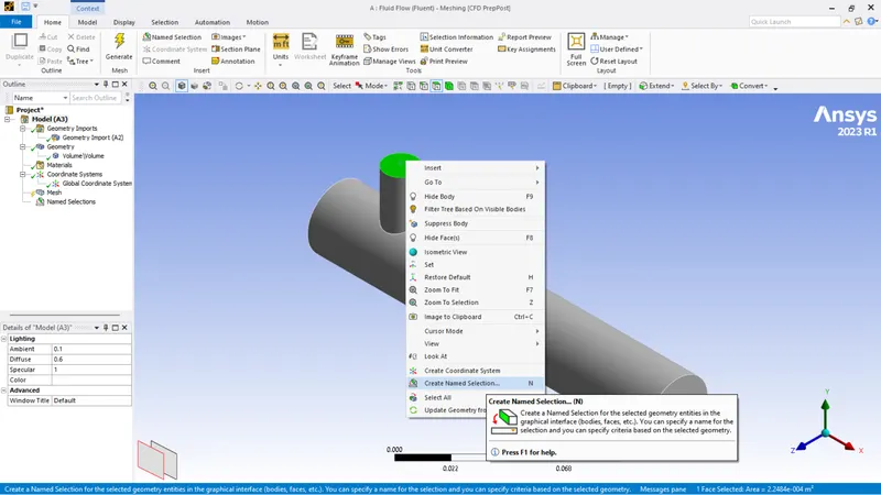
- Once we have named all the sections of the volume we can move onto the next steps.
Mesh Dependency test
- If you click on the mesh on the project path, we can see the details of the default mesh chosen by ansys using the boundary box technique. we can use this mesh quality to do a mesh dependency test.
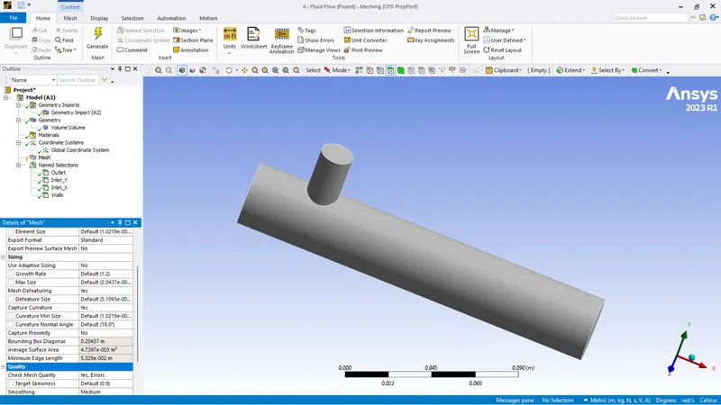
- Click on generate mesh to start the meshing process.
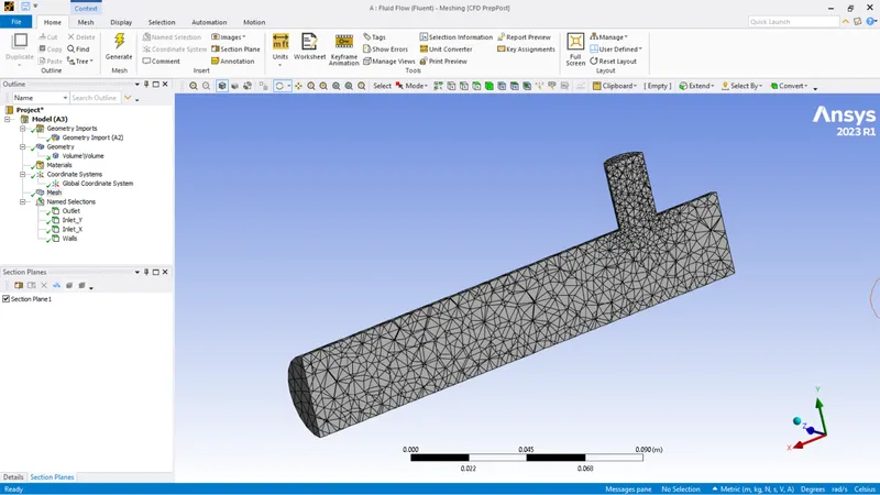
- Mesh - Nodes : 2825 & Elements : 12692 using default ansys meshing.
- Next we move onto setup.
| Solver Type | Pressure Based |
| Velocity Formulation |
Absolute |
| Time | Steady State |
| Energy | Energy is selected since temperature is required |
| Viscous model | Realizable K-epsilon with standard wall function |
| Material | Air |
| Cell Zone | Volume - air |
Boundary Conditions:
| Inlet_X | Velocity Inlet; Velocity Magnitude : 3 m/s; Thermal-Temperature : 36 degree celsius |
| Inlet_Y | Velocity Inlet; Velocity Magnitude : 6 m/s; Thermal-Temperature : 19 degree celsius |
| Wall | Wall-Stationary |
| Outlet | Pressure Outlet; Gauge pressure : 0 Pa; Thermal-Temperature : 26.85 degree celsius |
- Solution was initialized with hybrid initialization and number of iterations as 300
Result of Default mesh
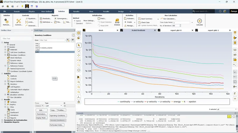
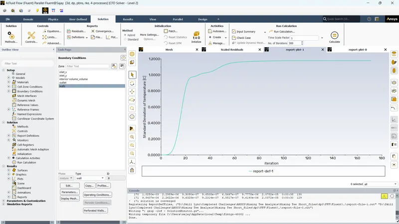
- The solution converged after 155 iterations
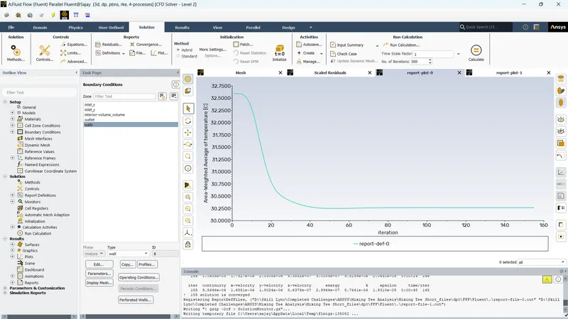
- Area weighted temperature at outlet - 30.2635 degree celsius
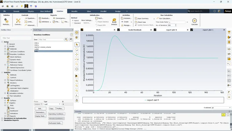
- Standard deviation at outlet - 1.1754
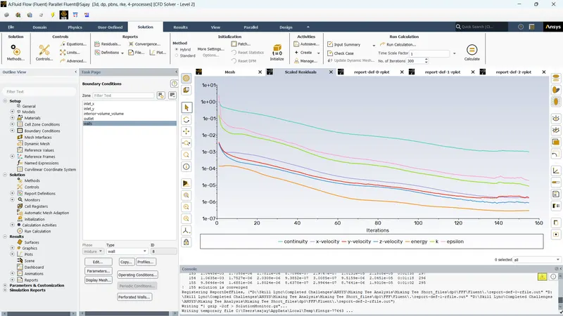
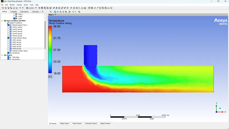
- Temperature contour along the Tee
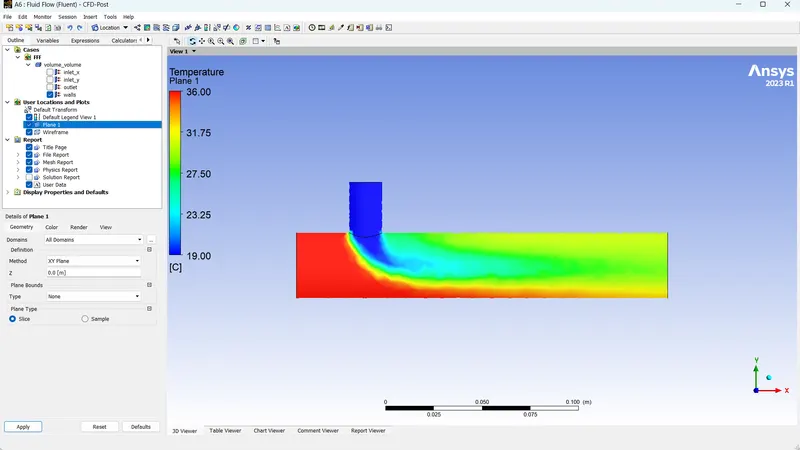
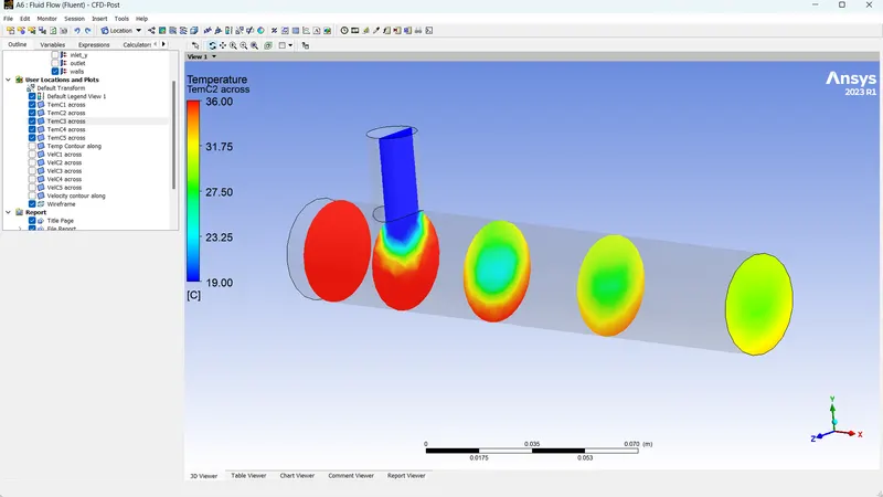
- Temp plot across Tee
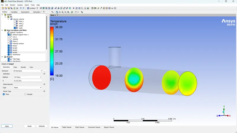
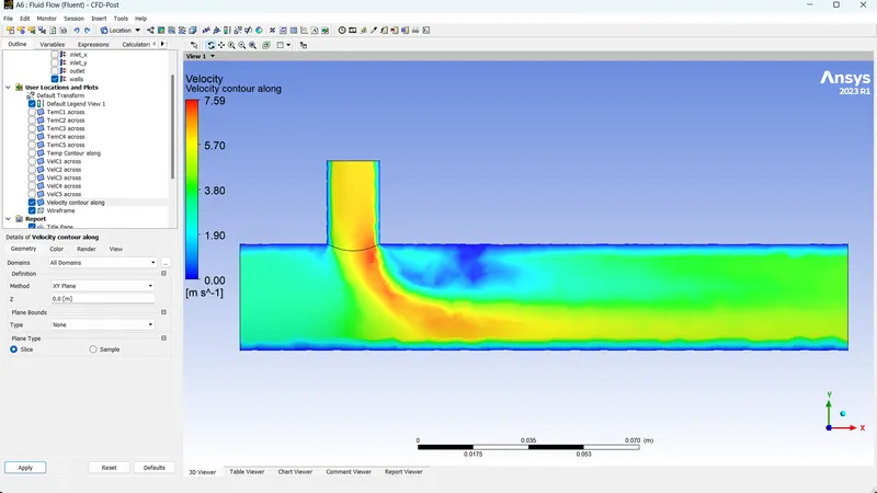
- Velocity contour along Tee
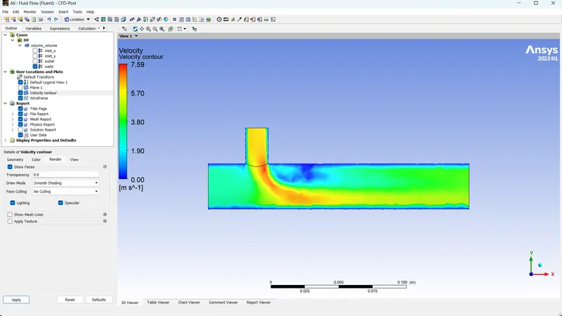
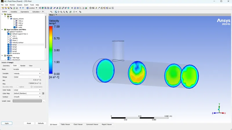
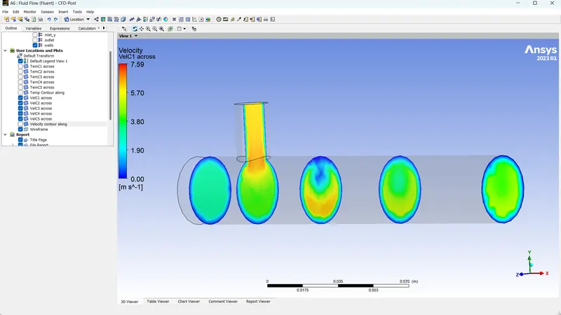
- Velocity contour across Tee
Mesh size Reduced
- The mesh element size was reduced to 0.002 m
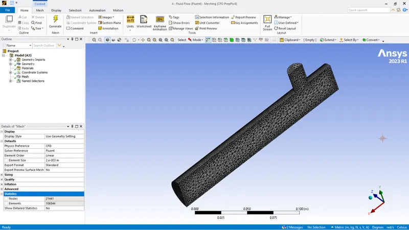
- Mesh - Nodes : 21441 & 106544
- Use the same setup and boundary conditions as mentioned above to initialize the solution.
Custom mesh Results
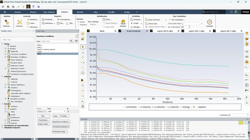
- The solution converged after 185 iterations.
- Area weighted temperature at outlet : 30.296 degree celsius
- Standard deviation of temperature at outlet : 1.845
- Residual plot of custom mesh
- Temperature contour along mixing Tee
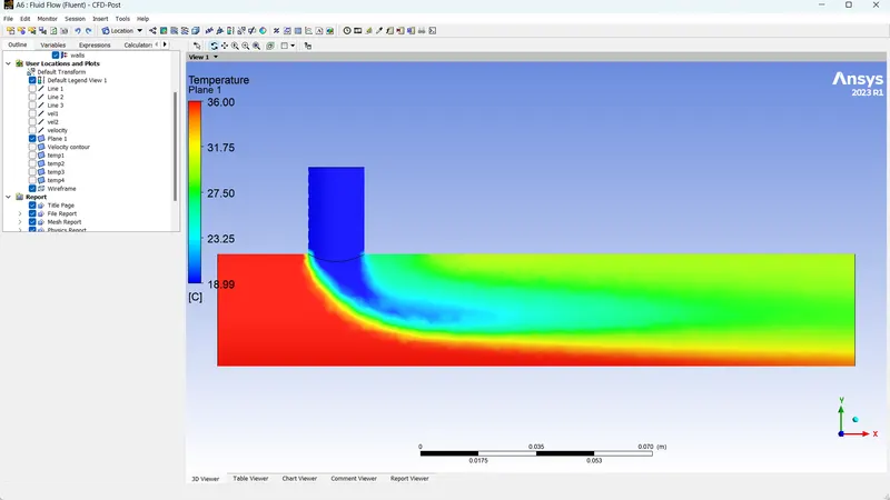
- Temperature contour across mixing tee
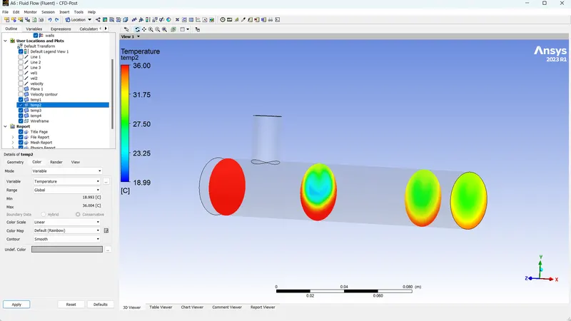
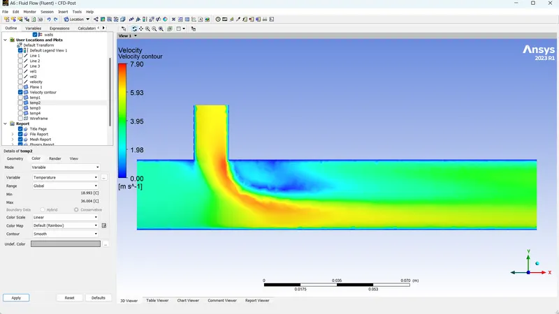
- Velocity contour along mixing Tee
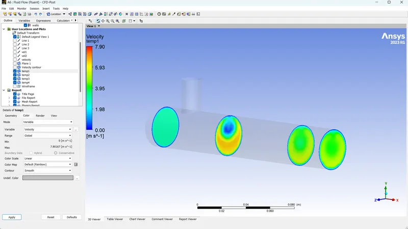
- Velocity contour across Tee
Mesh Dependency Test Conclusion
Mesh dependency test was done on the mixing tee with element size 0.01m and 0.002 m
| List | 0.01 m mesh | 0.002m mesh |
| Nodes | 2825 | 21441 |
| Elements | 12692 | 106544 |
| Iterations to converge | 155 | 185 |
| Area weighted temperature at outlet | 30.2635 degree celsius | 30.2960 degree celsius |
| Standard deviation of temperature at outlet | 1.1754 | 1.845 |
It is evident from the above table that decreasing the mesh size has no significant change in the output temperature calculations. The finer mesh takes longer to converge. So we can conclude that 0.01 m mesh size can be used for the analysis of the mixing tee with all the given cases.
Case 1 : Analysis of Short Mixing Tee
K-Epsilon Viscous model with Momentum Ratio 2
Mesh element size was chosen as 0.01 m from mesh dependency test. The solution was initialized with the following setup.
| Type | Pressure Based Solver |
| Velocity formulation | Absolute |
| Time | Steady state |
| Energy | Selected |
| Viscous Model | Realizable K-Epsilon model with standard wall function |
| Material | Air |
| Cell Zones | Air |
Boundary Conditions were given as follows
| Inlet_X | Velocity Inlet; Velocity Magnitude : 3 m/s; Thermal-Temperature : 36 degree celsius |
| Inlet_Y | Velocity Inlet; Velocity Magnitude : 6 m/s; Thermal-Temperature : 19 degree celsius |
| Wall | Wall-Stationary |
| Outlet | Pressure Outlet; Gauge Pressure : 0 Pa; Thermal-Temperature : 26.85 degree celsius |
The solution was initialized using hybrid initialization and 300 iterations were given for calculations.
Result K-Epsilon Viscous Model with Momentum Ratio 2
| Mesh Nodes | 2825 |
| Mesh Elements | 12692 |
| Number of iterations for solution convergence | 155 |
| Area weighted average temperature at outlet | 30.2635 degree celsius |
| Standard deviation of temperature at outlet | 1.1755 |
- Residuals Convergence graph
- Area weighted temperature graph
- Standard deviation graph
- Temperature contour along the mixing Tee
- Temperature contour across mixing Tee
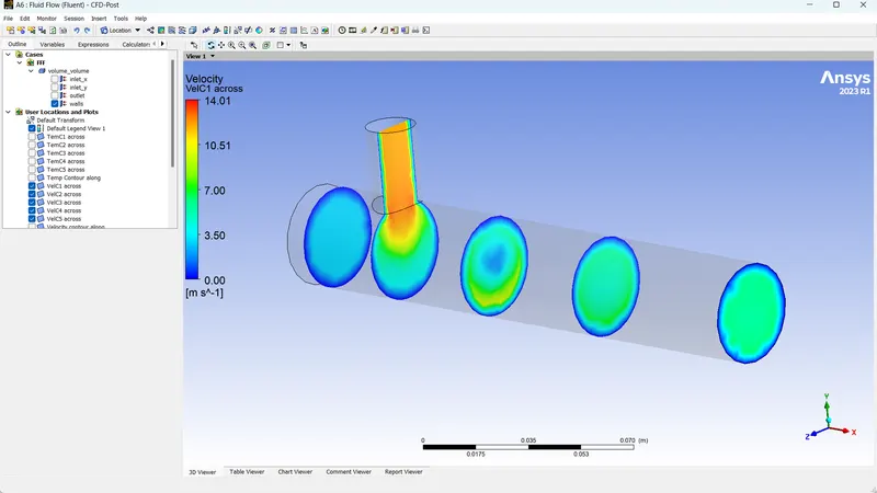
- Velocity contour along mixing Tee
- Velocity contour across mixing Tee
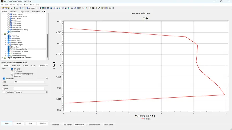
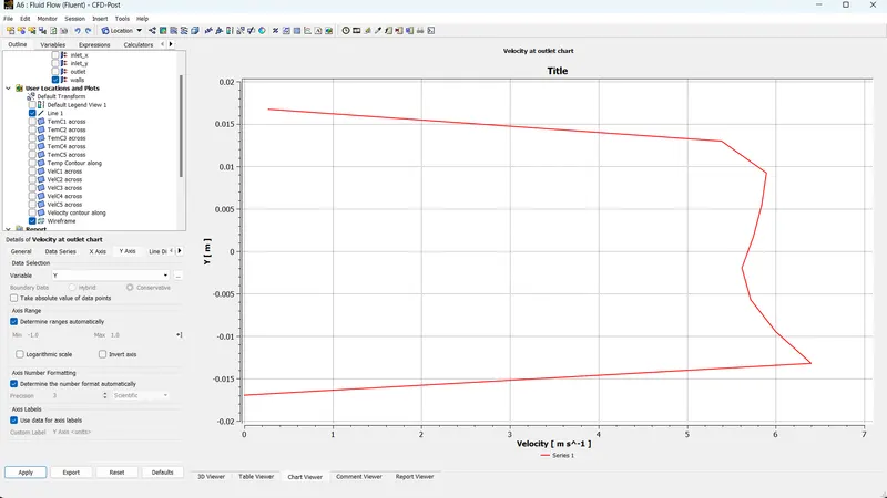
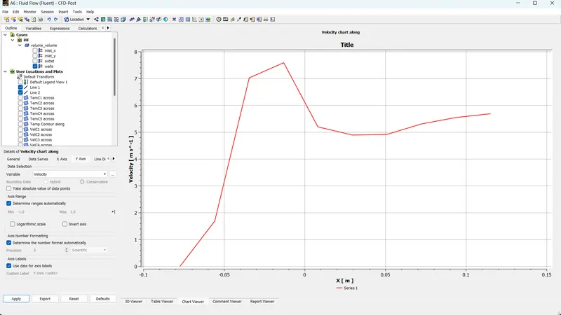
- Velocity chart at outlet
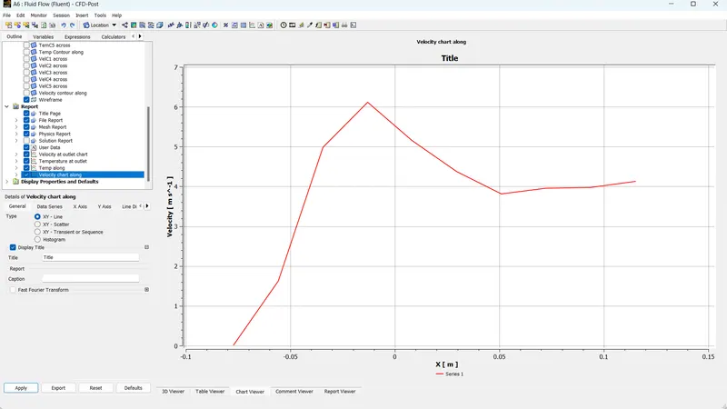
- Velocity chart along tee
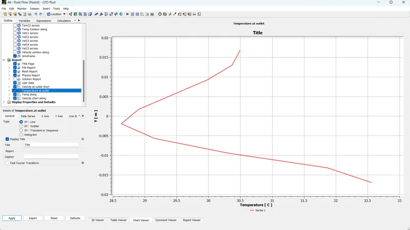
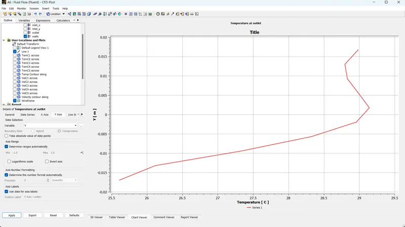
- Temperature chart at outlet
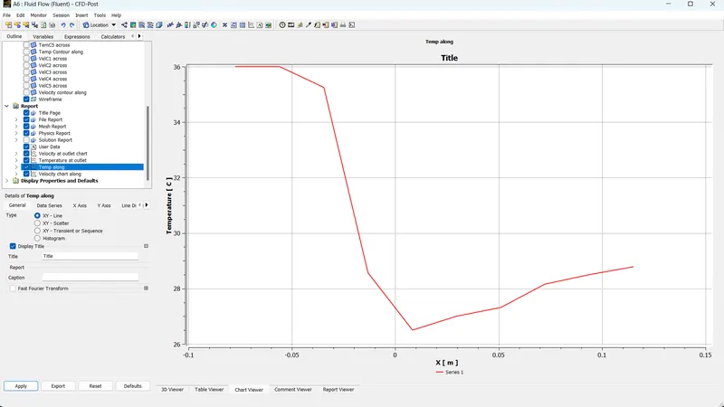
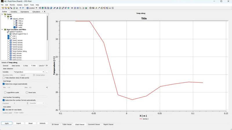
- Temperature chart along tee
K-Epsilon viscous Model with Momentum Ratio 4
The setup remained the same. Only Boundary Conditions were changed as follows
| Inlet_X | Velocity Inlet; Velocity Magnitude : 3 m/s; Thermal-Temperature : 36 degree celsius |
| Inlet_Y | Velocity Inlet; Velocity Magnitude : 12m/s; Thermal-Temperature : 19 degree celsius |
| Wall | Wall-Stationary |
| Outlet | Pressure Outlet; Gauge Pressure : 0 Pa; Thermal-Temperature : 26.85 degree celsius |
The solution was initialized using hybrid initialization and 300 iterations were given for calculations.
Result K-Epsilon Viscous Model with Momentum Ratio 4
| Mesh Nodes | 2825 |
| Mesh Elements | 12692 |
| Number of iterations for solution convergence | 171 |
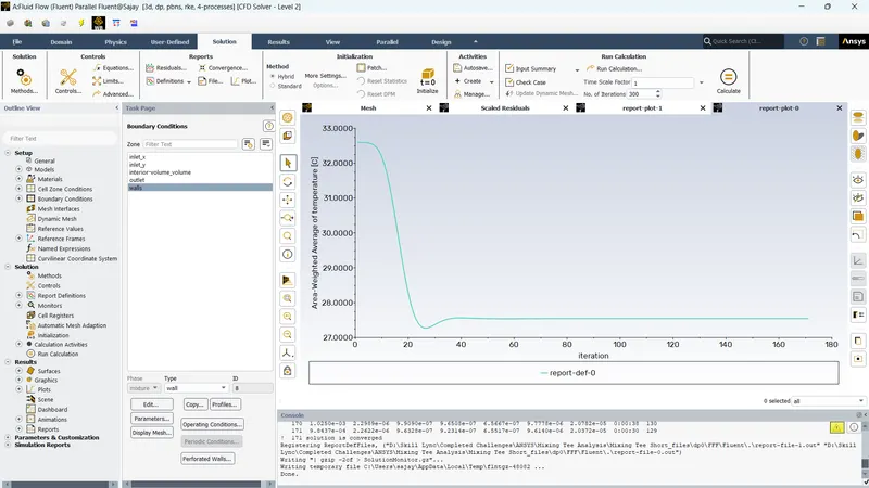
| Area weighted average temperature at outlet | 27.5434 degree celsius |
| Standard deviation of temperature at outlet | 1.1785 |
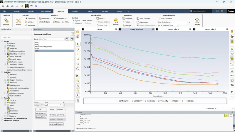
- Residual convergence graph
- Area weighted temperature plot
- Stadard deviation plot
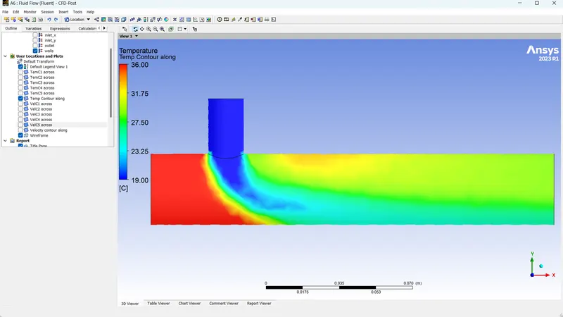
- Temperature contour along Tee
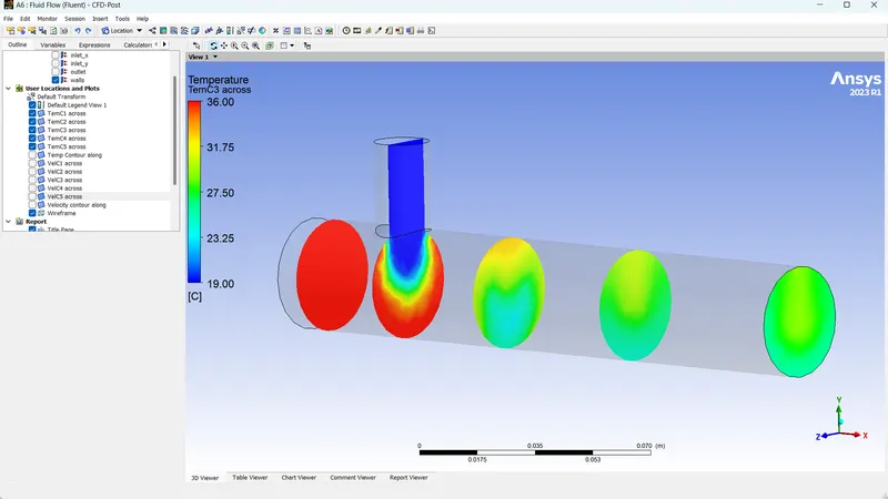
- Temperature contour across Tee
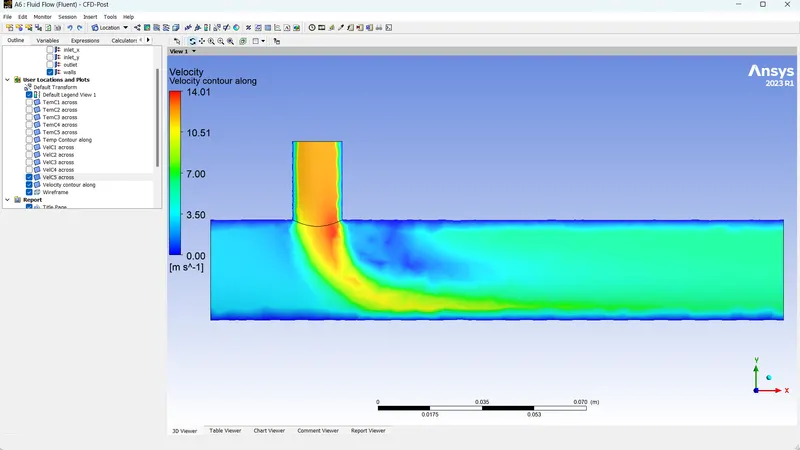
- Velocity Contour along Tee
- Velocity contour across Tee
- Velocity chart at outlet
- Temperature chart at outlet
- Temperature chart along the mixing tee
- Velocity chart along the mxing tee
Conclusion of K-Epsilon Model
| Item | Momentum Ratio 2 | Momentum Ratio 4 |
| Iterations for convergence | 155 | 171 |
| Area weighted average temperature at outlet | 30.26 degree celsius | 27.54 degree celsius |
| Standard deviation of temperature at outlet | 1.1755 | 1.1785 |
It is evident from the above table that the outlet temperature is reduced when the cold air inlet velocity is increased. Observation of the temperature and velocity contours shows better mixing and faster achievement of cooler temperature downstream of the two inlets when the cold air inlet velocity is increased.
K-Omega SST Viscous model with Momentum Ratio 2
Mesh element size was chosen as 0.01 m from mesh dependency test. The solution was initialized with the following setup.
| Type | Pressure Based Solver |
| Velocity formulation | Absolute |
| Time | Steady state |
| Energy | Selected |
| Viscous Model | K-Omega SST |
| Material | Air |
| Cell Zones | Air |
Boundary Conditions were given as follows
| Inlet_X | Velocity Inlet; Velocity Magnitude : 3 m/s; Thermal-Temperature : 36 degree celsius |
| Inlet_Y | Velocity Inlet; Velocity Magnitude : 6 m/s; Thermal-Temperature : 19 degree celsius |
| Wall | Wall-Stationary |
| Outlet | Pressure Outlet; Gauge Pressure : 0 Pa; Thermal-Temperature : 26.85 degree celsius |
The solution was initialized using hybrid initialization and 300 iterations were given for calculations.
Result K-Omega SST Viscous Model with Momentum Ratio 2
| Mesh Nodes | 2825 |
| Mesh Elements | 12692 |
| Number of iterations for solution convergence | Not converged |
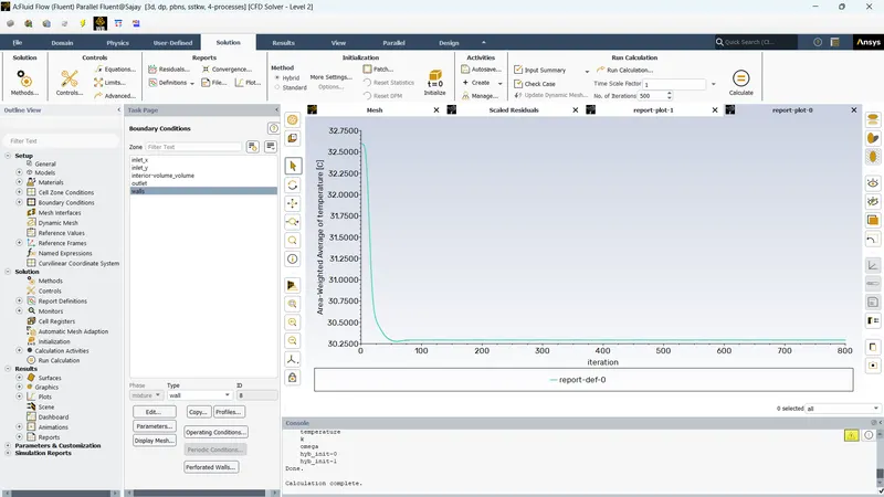
| Area weighted average temperature at outlet | 30.2934 |
| Standard deviation of temperature at outlet | 1.2 |
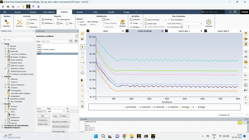
- Residual plot
- Area weighted temperature plot at outlet
- Standard deviation plot
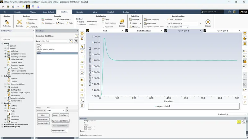
The solution did not converge even after 800 iterations but the outlet temperature at 800 iteration is 30.2934 degree celsius.
K-Epsilon viscous model was chosen over K-Omega model due to it's faster convergence and good results for further analysis.
Case 2 : Analysis of Long Mixing Tee
K-Epsilon Viscous model with Momentum Ratio 2
Mesh element size was chosen as 0.01 m from mesh dependency test. The solution was initialized with the following setup.
| Type | Pressure Based Solver |
| Velocity formulation | Absolute |
| Time | Steady state |
| Energy | Selected |
| Viscous Model | Realizable K-Epsilon model with standard wall function |
| Material | Air |
| Cell Zones | Air |
Boundary Conditions were given as follows
| Inlet_X | Velocity Inlet; Velocity Magnitude : 3 m/s; Thermal-Temperature : 36 degree celsius |
| Inlet_Y | Velocity Inlet; Velocity Magnitude : 6 m/s; Thermal-Temperature : 19 degree celsius |
| Wall | Wall-Stationary |
| Outlet | Pressure Outlet; Gauge Pressure : 0 Pa; Thermal-Temperature : 26.85 degree celsius |
The solution was initialized using hybrid initialization and 300 iterations were given for calculations.
Result K-Epsilon Viscous Model with Momentum Ratio 2
| Mesh Nodes | 3479 |
| Mesh Elements | 15635 |
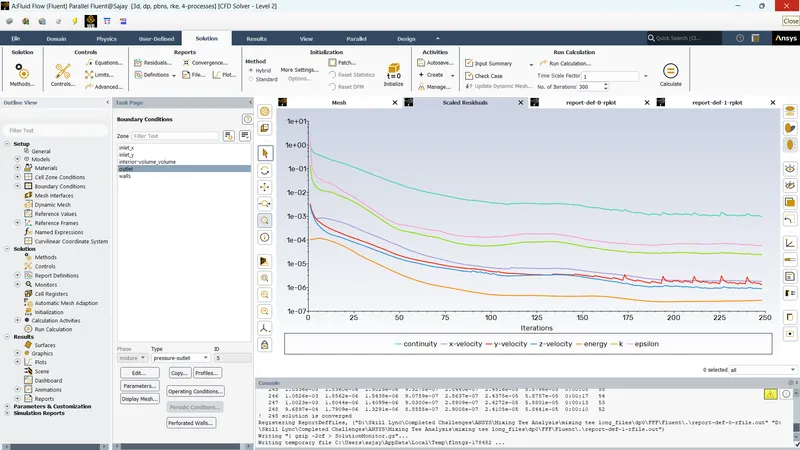
| Number of iterations for solution convergence | 248 |
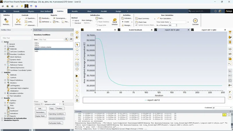
| Area weighted average temperature at outlet | 30.2468 degree celsius |
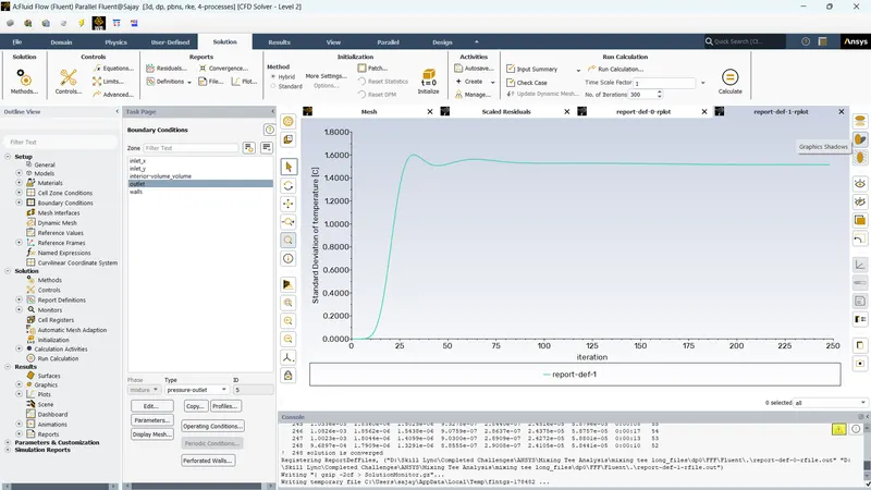
| Standard deviation of temperature at outlet | 1.5149 |
- Residual chart
- Standard deviation of temperature at outlet
- Area weighted temperature of outlet
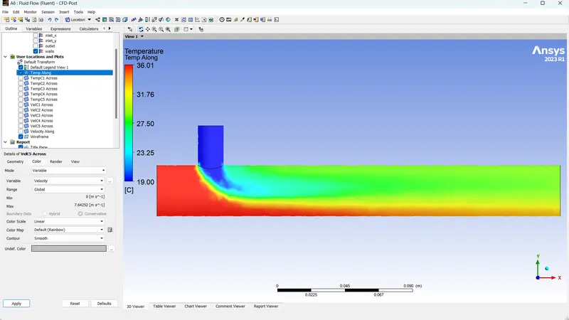
- Temperature contour along tee
- Temperature contour across tee
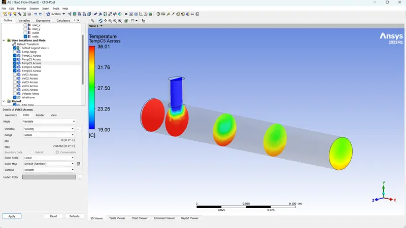
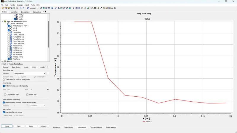
- Temperature chart along tee
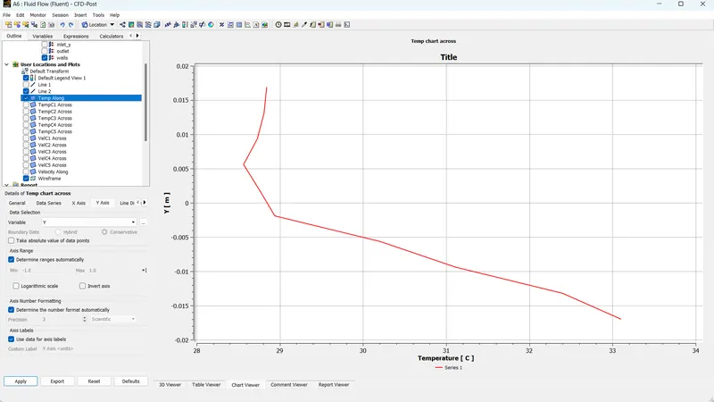
- Temperature chart across tee
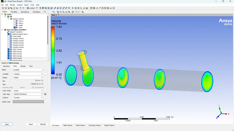
- Velocity contour along tee
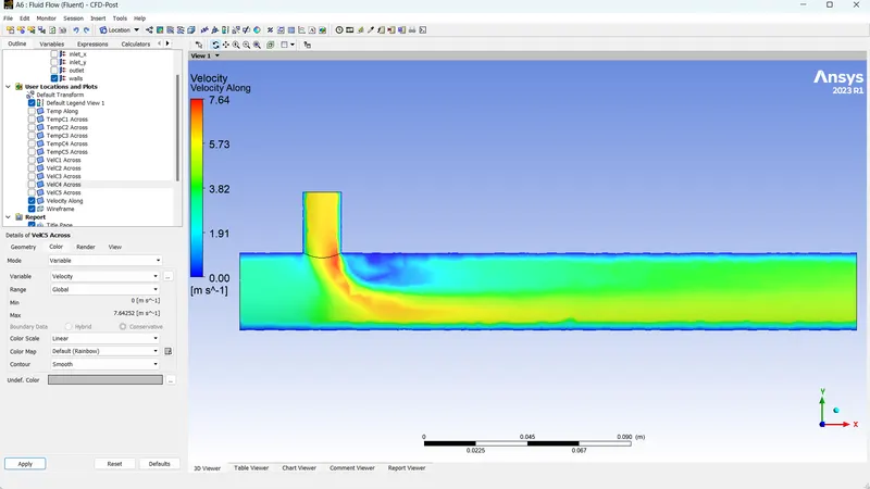
- Velocity contour across tee
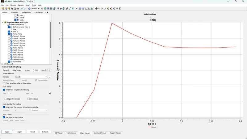
- Velocity chart along tee
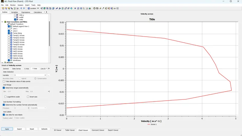
- Velocity chart across tee
K-Epsilon viscous Model with Momentum Ratio 4
The setup remained the same. Only Boundary Conditions were changed as follows
| Inlet_X | Velocity Inlet; Velocity Magnitude : 3 m/s; Thermal-Temperature : 36 degree celsius |
| Inlet_Y | Velocity Inlet; Velocity Magnitude : 12m/s; Thermal-Temperature : 19 degree celsius |
| Wall | Wall-Stationary |
| Outlet | Pressure Outlet; Gauge Pressure : 0 Pa; Thermal-Temperature : 26.85 degree celsius |
The solution was initialized using hybrid initialization and 300 iterations were given for calculations.
Result K-Epsilon Viscous Model with Momentum Ratio 4
| Mesh Nodes | 2825 |
| Mesh Elements | 12692 |
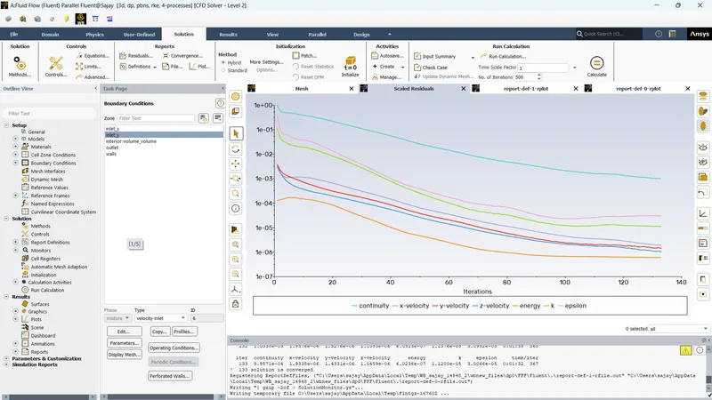
| Number of iterations for solution convergence | 133 |
| Area weighted average temperature at outlet | 27.4915 degree celsius |
| Standard deviation of temperature at outlet | 0.5356 |
- Residual plot
- Area weighted temperature plot at outlet
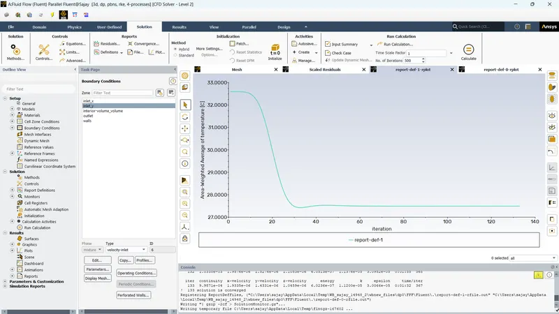
- Standard deviation of temperature at outlet
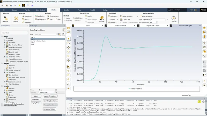
- Temperature contour along tee
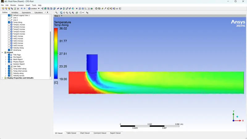
- Temperature contour across tee
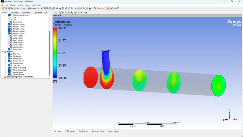
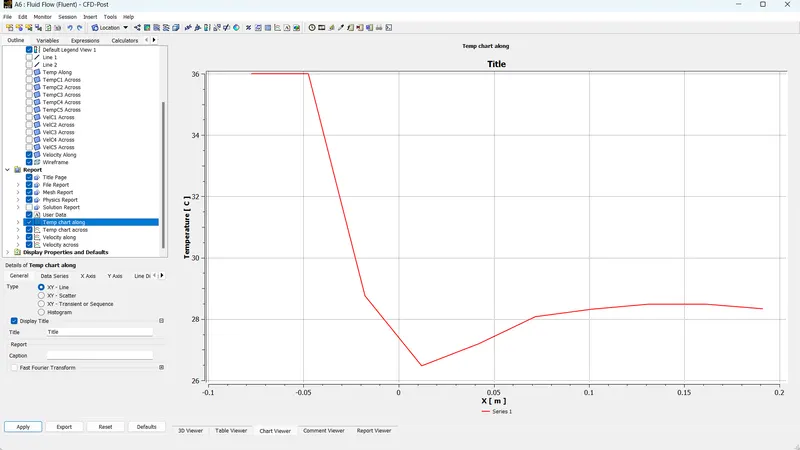
- Temperature chart along tee
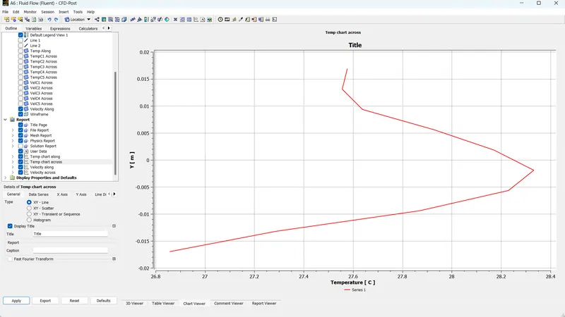
- Temperature chart across tee
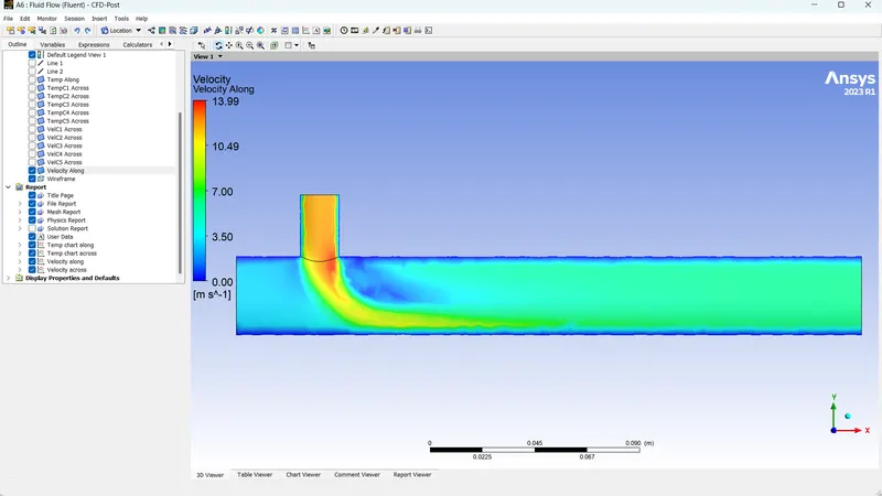
- Velocity contour along tee
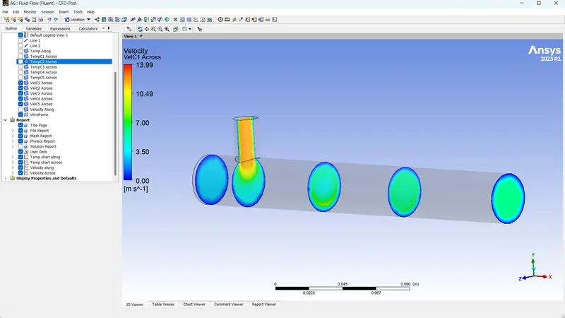
- Velocity contour across tee
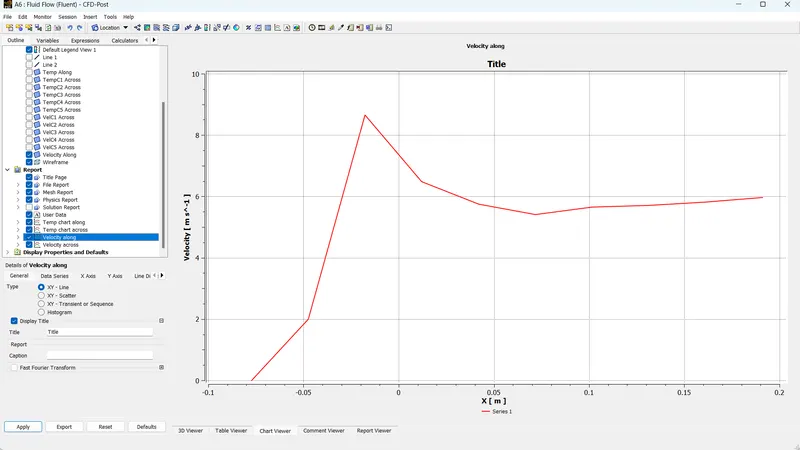
- Velocity chart along tee
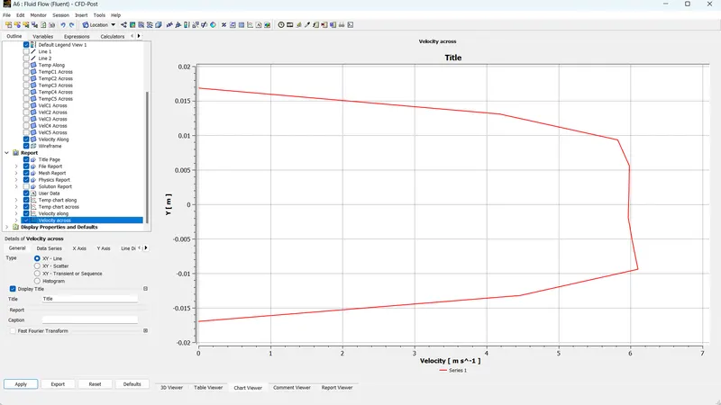
- Velocity chart across tee
Conclusion of K-Epsilon Model long mixing tee
| Item | Momentum Ratio 2 | Momentum Ratio 4 |
| Iterations for convergence | 248 | 133 |
| Area weighted average temperature at outlet | 30.24 degree celsius | 27.49 degree celsius |
| Standard deviation of temperature at outlet | 1.5149 | 0.5356 |
Lower temperature is achieved at the outlet when cold air inlet velocity is increased. It is also observed that the fluids are more uniformly mixed downstream when the cold air inlet velocity is increased.
Comparison of short and long mixing tee
| Items | Short Mixing Tee | Long Mixing Tee |
| Mesh nodes | 2825 | 3479 |
| Mesh Elements | 12692 | 15635 |
| Average iterations for convergence | 163 | 191 |
| Average outlet temperature | 28.9 degree celsius | 28.86 degree celsius |
Conclusion
We can conclude that increasing the cold air inlet velocity has a more significant effect on reducing the outlet temperature. Increasing the length of the mixing tee has not much significant effect in reducing the outlet temperature. However, the flow becomes more uniform as we increase the length of the mixing tee which is evident from the graphs and pictures provided in the result sections.
If decreasing the outlet temperature is the sole concern, increasing the velocity of cold air inlet helps achieving the result.