Week 1- Mixing Tee
Aim : To set up steady-state simulations to compare the mixing effectiveness when the hot inlet temperature is 36 °C and the cold inlet temperature is 19 °C.
Objective : To set up steady-state simulations to compare the mixing effectiveness when the hot inlet temperature is 36 °C and the cold inlet temperature is 19 °C.
- Figure out the more suitable case between k-epsilon and k-omega SST models.
- Case 1
- Short mixing tee with a hot inlet velocity of 3m/s.
- Momentum ratio of 2, 4.
- Case 2
- Long mixing tee with a hot inlet velocity of 3m/s.
- Momentum ratio of 2, 4.
-
Compare the following values from the 2 cases.
- Cell count
- Average outlet temperature
- Number of iterations for convergence
Expected results:
- Velocity and temperature contour plots on the cut planes along and across the pipe.
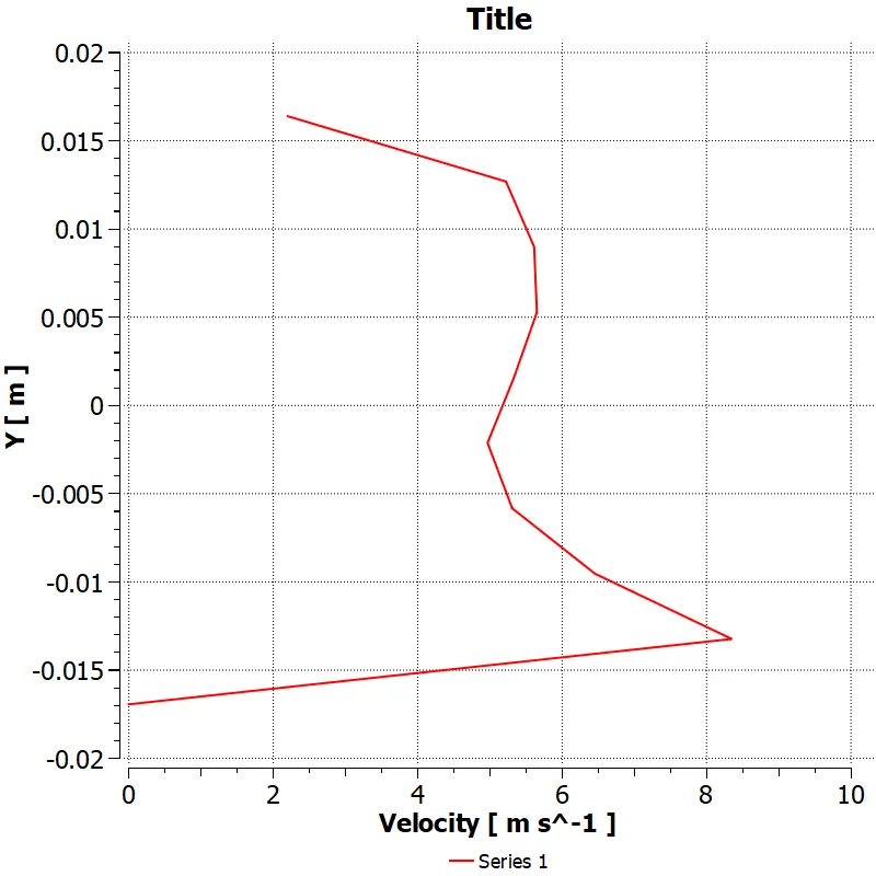
- Velocity and temperature line plots along and across the length of the pipe.
- Perform Mesh independent study for any one case.
- Discuss the effect of length and momentum ratio on results.
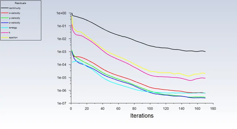
For each simulation, we need to show the convergence plot
Introduction :
For making accurate predictions of near-wall, the mesh resolution and modeling approach are equally important. The model of choice and the grid resolution are tightly coupled in the sense that a very good model for a specific application will achieve acceptable predictions only if the mesh resolution matches the chosen specific model.
This model is essentially a high Reynolds number model, meaning the law of the wall must be employed and provide velocity "boundary conditions" away from solid boundaries (what is termed "wall-functions"). Another major drawback is the model's lack of sensitivity to adverse pressure-gradient. It was observed that under such conditions it overestimates the shear stress and by that delays separation.
This model is essentially a low Reynolds number model. This model takes 'elliptic' near-wall behavior meaning that it has an inherent nature of being able to "communicate" with the wall and actually has Dirichlet (as in no-slip in this case) boundary conditions. The implication of such behavior is the straightforward possibility of integrating through the laminar sublayer without additional numerically destabilizing damping functions or two additional transport equations.
Geometry Cleanup
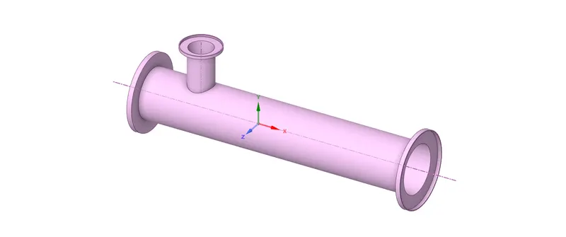
Here is our raw Cad geometry that we have received. So the first and foremost thing is to clean up the geometry for our CFD simulation purposes.
Here we are interested in internal flow analysis, so we don't need those extra thicknesses present in our geometry and we need to extract our Fluid Volume
For this we can perform Fluid Extraction Operation
Prepare -> Volume Extraction -> Select edges -> Supress for physics( so that the extra thickness doesnt generate mesh)
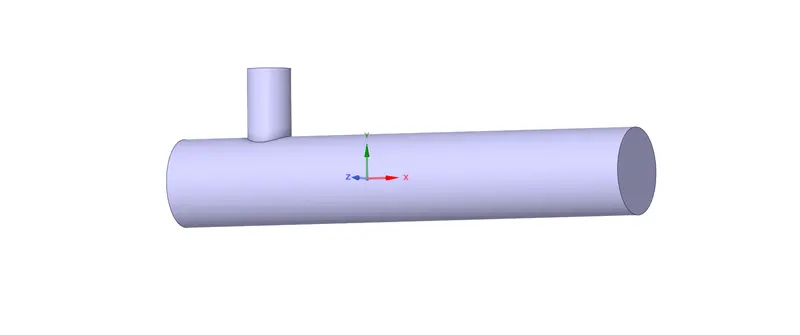
Now we should move to our Meshing Module from Workbench Screen
Mesh Generation
For perfoming CFD Simulations, first of all we need to define inlet outlet and boundary conditions on our respective geometry.
For this we can perform Named Selection Operation
Smart Select -> Select the respective edge -> Hit "N" Shorcut key for Named Selection -> Provide Appropiate Naming
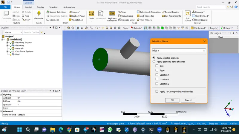
Now, we finally move to Mesh Generation Process
For mesh generation, we are currently using the default mesh generation process
Mesh -> Right Click -> Generate Mesh which will generate mesh over the whole body with pre-defined values

Mesh Sizing
| Cells | Faces | Nodes |
|
12692 |
26679 | 2825 |
Now we need to analyse our mesh generated using Mesh Metric -> Element Quality

We can observe that our element size is not below 31% (0.31), which is way away from the limiting value of 5%..So we can move forward with the current mesh generated over our geometry.
With these our work is completed in Mesh Tab and we can move forward to Setup tab for further operations.
After entering into our Fluent Screen, the first thing we need to do is check our mesh quality
Mesh -> Perform Mesh Check -> Check the status on Console Screen
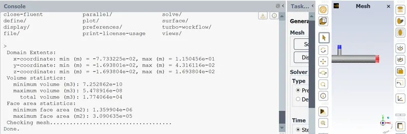
Here, we cant find any warning related to our mesh generation, so we can finalize the mesh and move forward to next deck.
Solving Steps
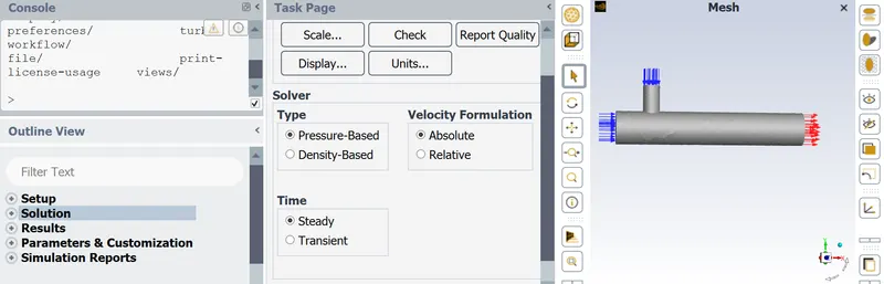
- Time -> Steady State
- Solver Type -> Pressure Based Solver ( For small Mach No.)
- Velocity Formulation -> Absolute
- And Select Energy Equation for obtaining Temperature
- For Viscous Model -> K epsilon -> Realizable -> Standard wall functions to capture the turbulent nature of flow.
- For Material -> Air
- Now we need to assign boundary conditions for performing our CFD Simulations and assign values of velocity and temperature as stated above at inlet conditions
- Before calculating our Results we need to run Initialize our solution which will create some guess values for smooth calculations.
- We can perform this operation using Solution -> Initialization -> Hybrid -> Set No of Iterations -> Run Initialization
- Now after Initialization we can finally Run our Calculations.
- We can perform this operation using Solution -> Run Calculation -> Time Scale Factor ( i.e 1) -> No of Iterations ( say 500 iterations) -> Hit on Calculate.
Input & Output Results Analysis using K-Epsilon Turbulence Model:
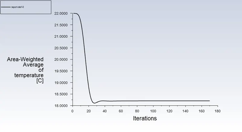
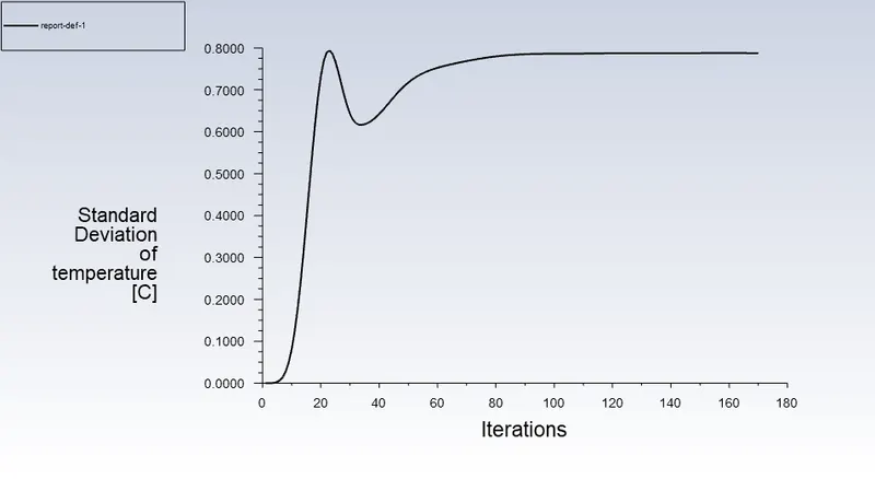
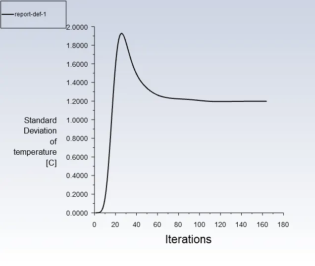
Here is our initial velocity and temperature listed along with the calculated result value of the average outlet temperature and standard deviation.
| Velocity Inlet-x(m/s) | Velocity Inlet-y(m/s) | Temperature Inlet-x(C) | Temperature Inlet-y(C) | Average Outlet Temperature(C) | Standard Deviation | Iterations for converge |
| 3 | 10 | 25 | 10 | 18.20 | 0.79 | 166 |
Solver Results :
Post-Processing Results
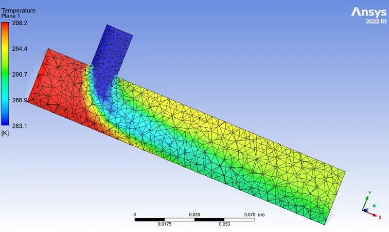
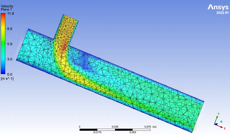
Input & Output Results Analysis using K Omega Model :
| Velocity at inlet-x(m/s) | Temperature at inlet-x(c) | Velocity at inlet-y(m/s) | Temperature at inlet-y(c) | Average outlet temperature(c) | Standard Deviation at outlet | Iterations for converge |
| 3 | 36 | 6 | 19 |
30.29446 |
1.1980117 |
162 |
Solver Results :
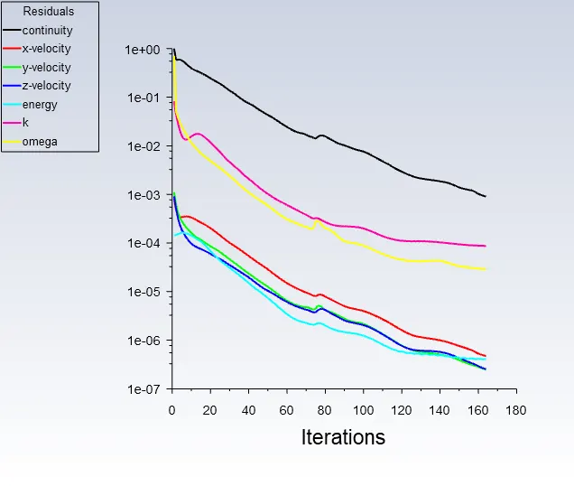
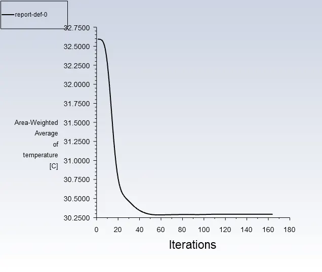
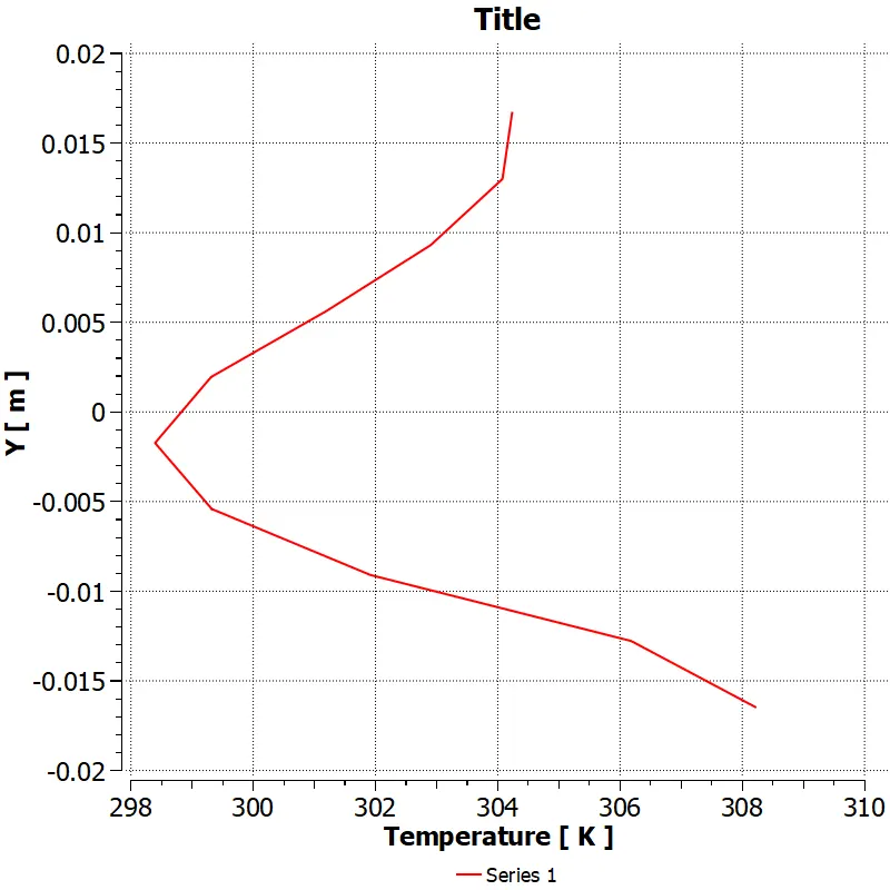
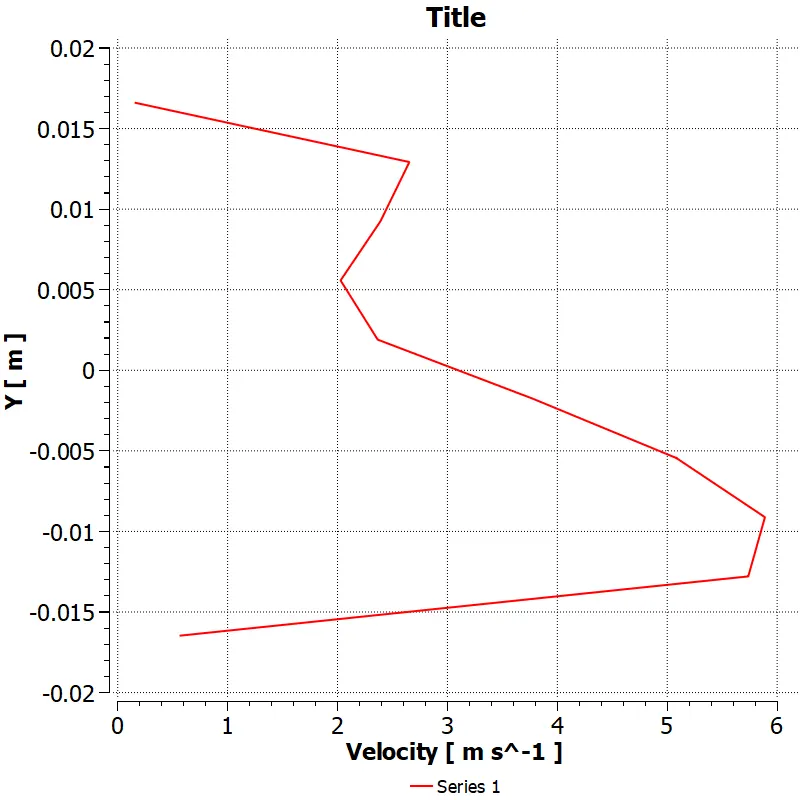
Note : We can conclude from the above contour plots that the results for both turbulence techniques are relatively close enough so we are choosing K-epsilon over K-omega for the further results.
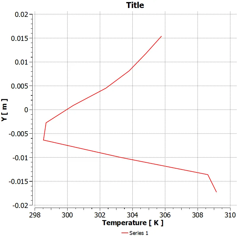
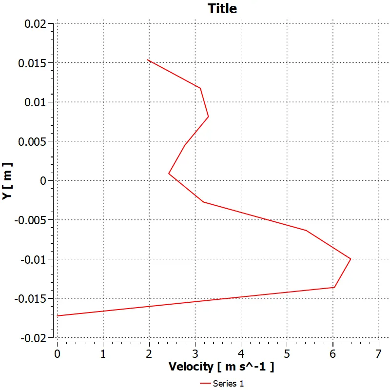
Case 1 :
- Short mixing tee with a hot inlet velocity of 3m/s.
- Momentum Ratio of 2
Input & Output Results Analysis using K-Epsilon Model :
| Velocity at inlet-x(m/s) | Temperature at inlet-x(c) | Velocity at inlet-y(m/s) | Temperature at inlet-y(c) | Average outlet temperature(c) | Standard Deviation at outlet | Iterations for converge |
| 3 | 36 | 6 | 19 |
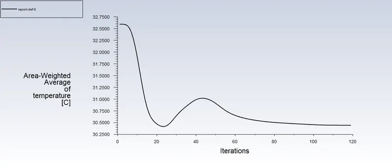
30.444436 |
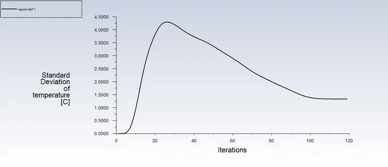
1.330798 |
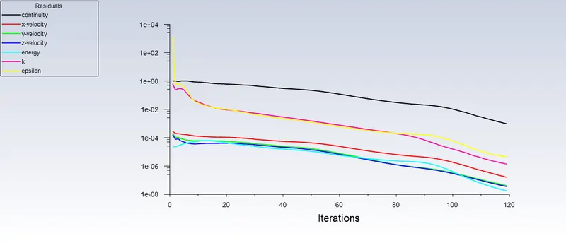
119 |
Solver Results
Post Processing Results
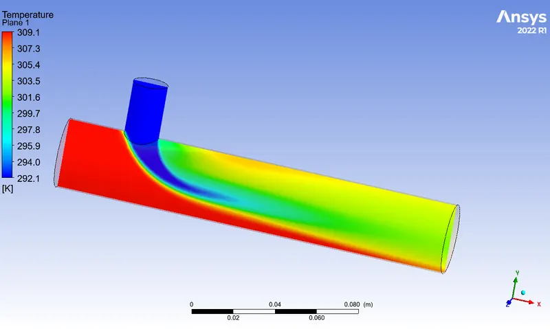
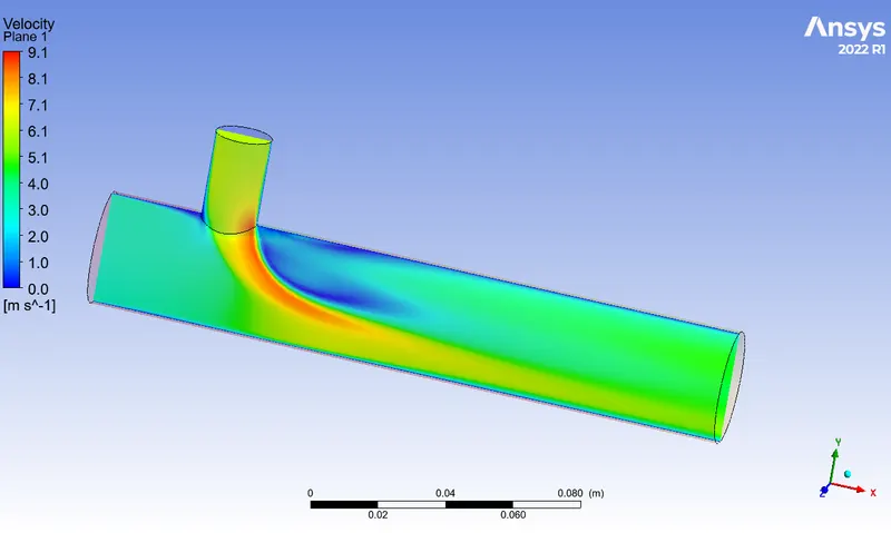
Case 1
- Short mixing tee with a hot inlet velocity of 3m/s.
- Momentum Ratio of 4
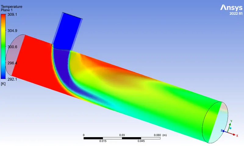
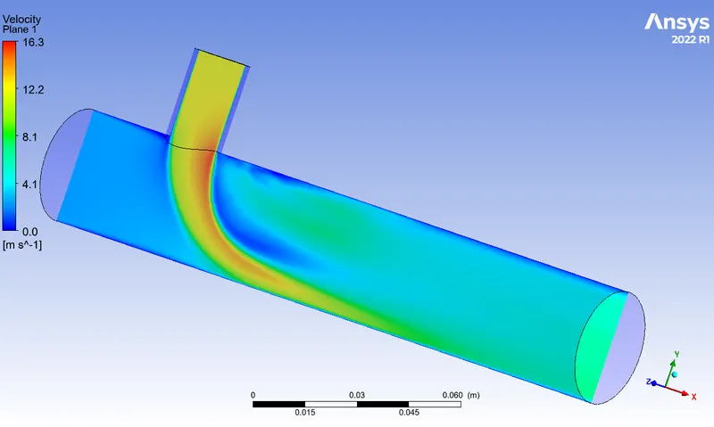
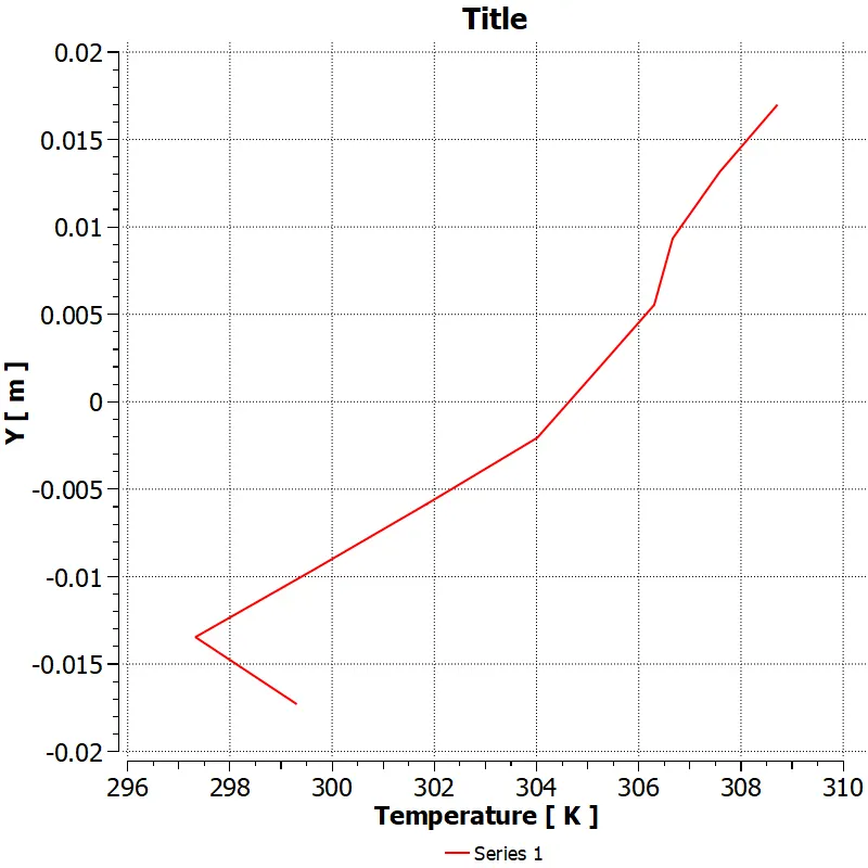
Input & Output Results Analysis using K-Epsilon Model :
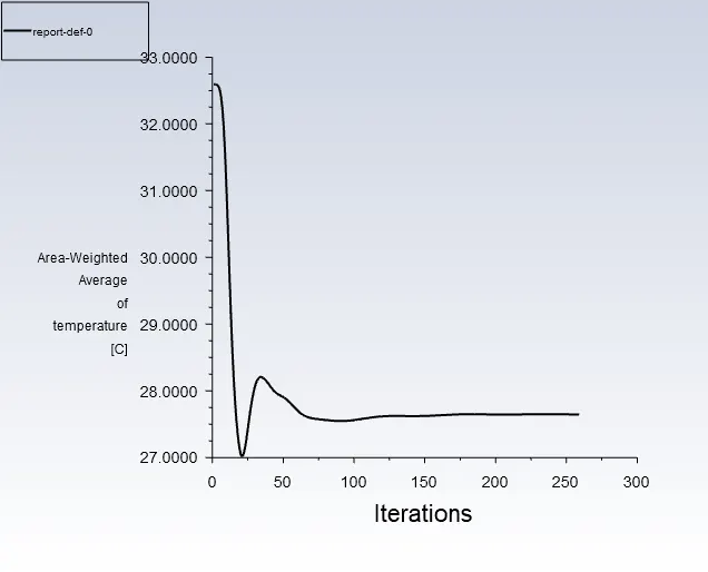
| Velocity at inlet-x(m/s) | Temperature at inlet-x(c) | Velocity at inlet-y(m/s) | Temperature at inlet-y(c) | Average outlet temperature(c) | Standard Deviation at outlet | Iterations for converge |
| 3 | 36 | 12 | 19 |
27.646572 |
1.6968748 |
259 |
Solver Results
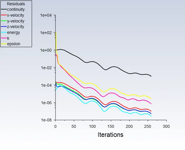
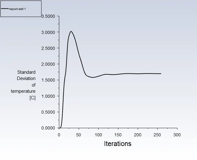
Post Processing Results
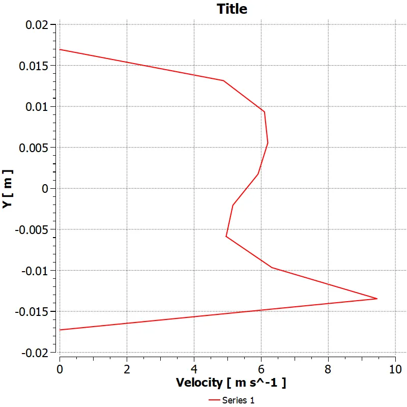
Case 2 :
- Long mixing tee with a hot inlet velocity of 3m/s.
- Momentum ratio of 2
Input & Output Results Analysis using K-Epsilon Model:
| Velocity at inlet-x(m/s) | Temperature at inlet-x(c) | Velocity at inlet-y(m/s) | Temperature at inlet-y(c) | Average outlet temperature(c) | Standard Deviation at outlet | Iterations for converge |
| 3 | 36 | 6 | 19 |
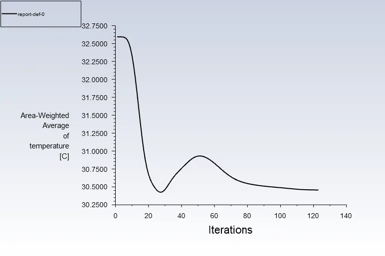
30.456813 |
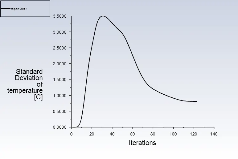
0.80962946 |
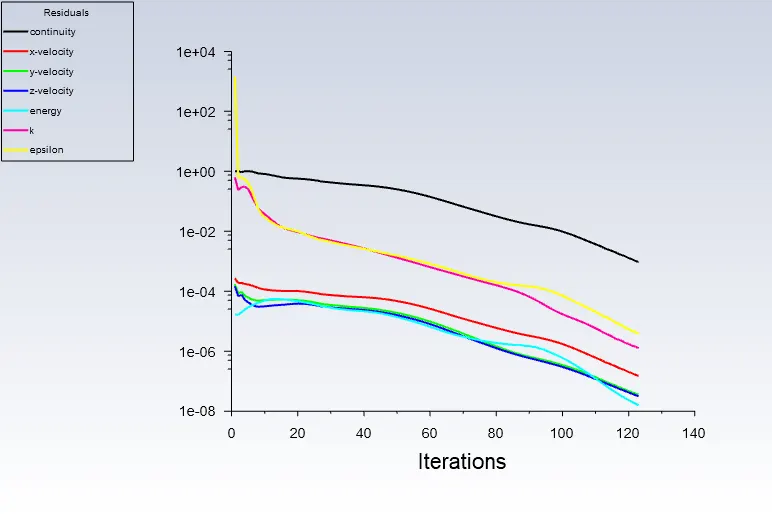
123 |
Solver Results
Pre-Processing Results
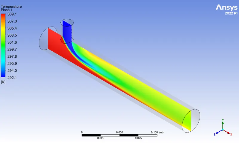
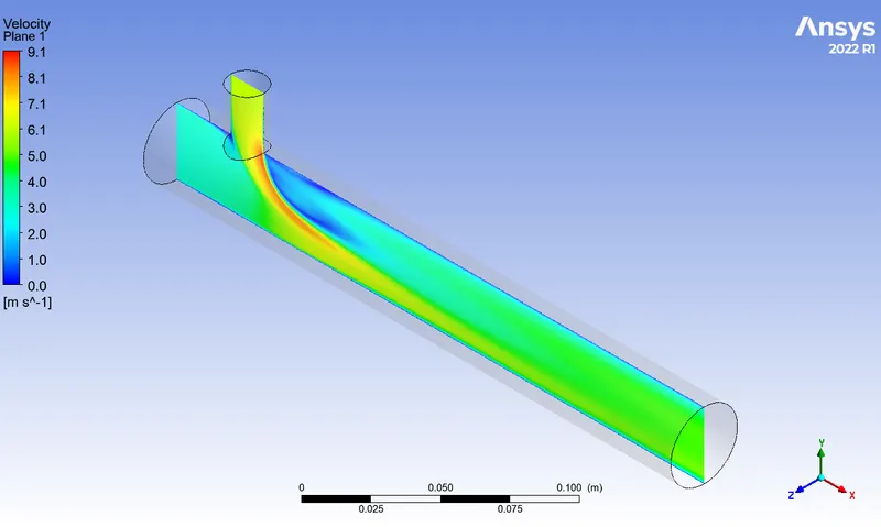
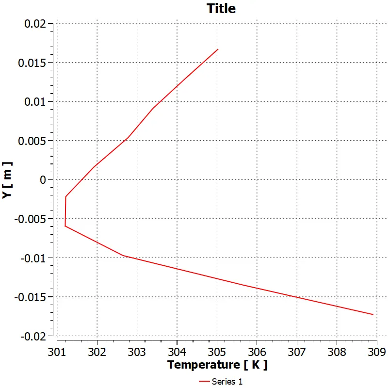
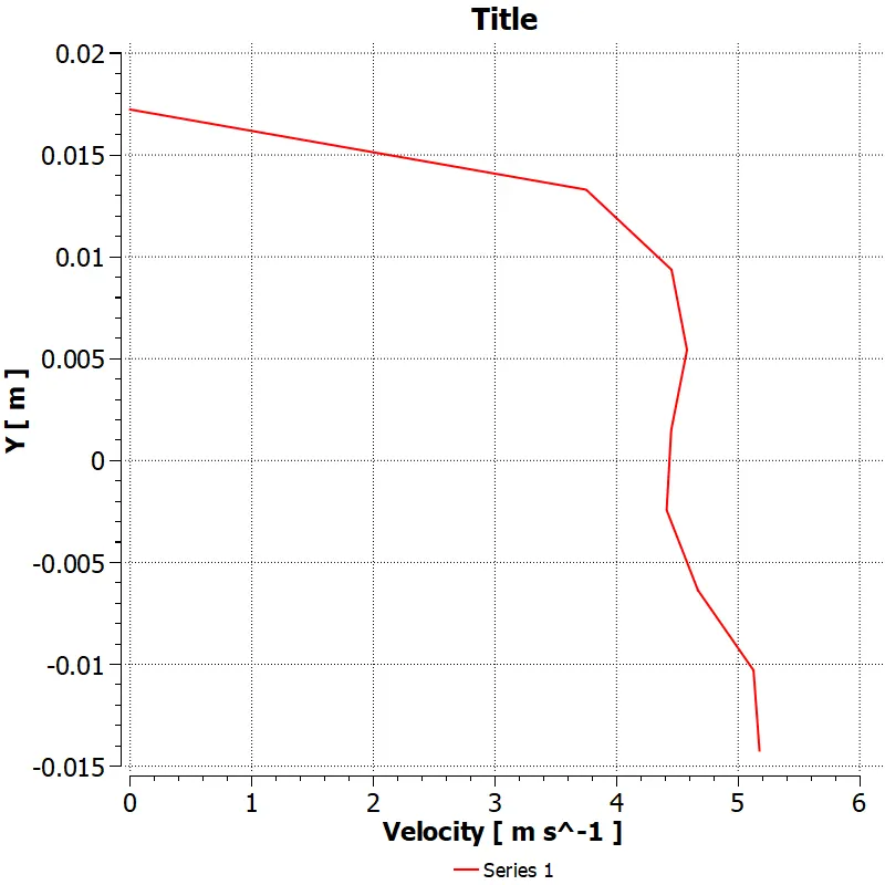
Case 2 :
- Long mixing tee with a hot inlet velocity of 3m/s.
- Momentum ratio of 4
Input & Output Results Analysis using K-Epsilon Model :
| Velocity at inlet-x(m/s) | Temperature at inlet-x(c) | Velocity at inlet-y(m/s) | Temperature at inlet-y(c) | Average outlet temperature(c) | Standard Deviation at outlet | Iterations for converge |
| 3 | 36 | 12 | 19 |
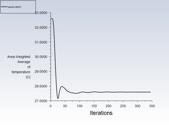
27.592297 |
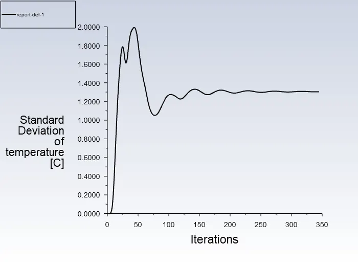
1.3038681 |
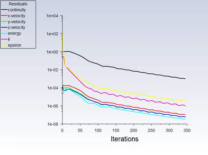
345 |
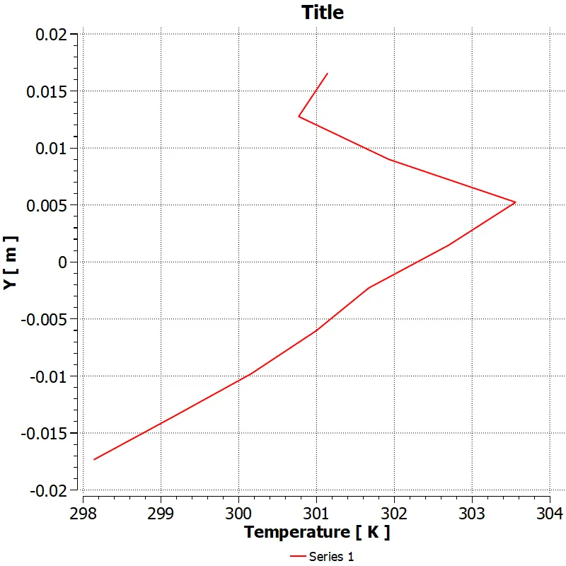
Solver Results
Results Comparision of all the cases
| Cases of Mixing Tee | Velocity at inlet-x(m/s) | Temperature at inlet-x(°c) | Velocity at inlet-y(m/s) | Temperature at inlet-y(°c) | Average outlet temperature(°c) | Standard Deviation at outlet |
| Coarse Mesh Short Tee Simulation with momentum ratio of 2 using K-Epsilon | 3 | 36 | 6 | 19 |
30.2672 |
1.1530898 |
| Coarse Mesh Short Tee Simulation with momentum ratio of 2 using K-Omega | 3 | 36 | 6 | 19 |
30.294492 |
1.197879 |
| Short Tee with momentum ratio of 2 | 3 | 36 | 6 | 19 | 30.444436 | 1.330798 |
| Short tee with momentum ratio of 4 | 3 | 36 | 12 | 19 | 27.646572 | 1.6968748 |
| Long tee with momentum ratio of 2 | 3 | 36 | 6 | 19 | 30.456813 | 0.80962946 |
| Long tee with momentum ratio of 4 | 3 | 36 | 12 | 19 | 27.592297 | 1.3038681 |
Meshing Details :
| Simulation Type | Element Sizing(mm) | Cells | Faces | Nodes |
|
Coarse Mesh Generation |
10 |
12692 |
26679 | 2825 |
| Short-Mixing-Tee | 0.5 | 3124910 | 6362295 | 578904 |
| Long-Mixing-Tee | 0.5 |
4275743 |
8703020 | 790899 |
Conclusion :
1. On comparing coarse mesh short-tee simulation with fine-tuned mesh short-tee simulation, we didn't get a huge change in results, but fine-tuned meshing increases computing time and requires a heavy computing system too.
2. Here we had to choose between K-Epsilon and K-omega SST Models, so here we are going with K-Epsilon Models as in fine-tune mesh simulations K-epsilon got convergence faster than the K-omega SST model. So for similar results, we should go with the one that is converging faster.
3. Here we cannot see any effect of length or momentum ratio on our final results. It could have also been figured out from our reference formula also, as it doesn't contain any length terms in it.