Week 1- Mixing Tee

Mixing Tee

AIM: To perform the steady-state simulations to compare the mixing effectiveness when hot inlet temperature is 36⁰C & the Cold inlet is at 19⁰C. For two different models under different cases.

OBJECTIVE:

To Use the k-epsilon and k-omega SST model for the first case and based on your judgment use the more suitable model for further cases. Giving the reason for choosing a suitable model is compulsory.

1. Case 1
   • Short mixing tee with a hot inlet velocity of 3m/s.
   • Momentum ratio of 2, 4.
2. Case 2
   • Long mixing tee with a hot inlet velocity of 3m/s.
   • Momentum ratio of 2, 4.

Momentum ratio = velocity at cold inlet / velocity at hot inlet

In a table, compare the following values from the 2 cases.

1. Cell count
2. Average outlet temperature
3. Number of iterations for convergence

Expected results:

1. Velocity and temperature contour plots on the cut planes along and across the pipe.
2. Velocity and temperature line plots along and across the length of the pipe.
3. Perform Mesh independent study for any one case.
4. Discuss the effect of length and momentum ratio on results.

INTRODUCTION:

In this week, we are going to perform the steady-state simulations to compare the mixing effectiveness when hot inlet temperature is 36⁰C & the Cold inlet is at 19⁰C. For two different models under different cases.

Mixing Tee which means a T-joint used in the pipelines of household and industries for flow of air/fluid. Its mechanism is to mix the two fluid flows in the perpendicular direction. This mechanism is used in A/C for hot and cold air for mixing efficiency to make comfortable inside the air-conditioned room.

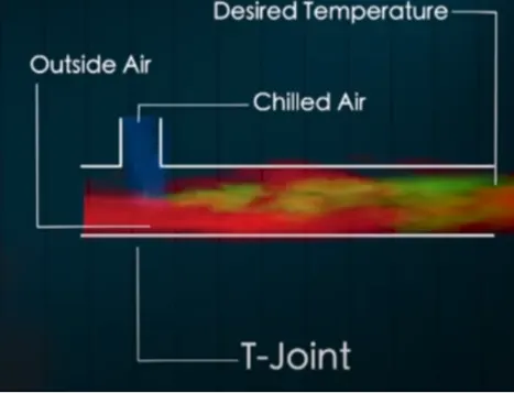
Example Figure

Steps involved in analysis:

• Pre-processing
• Solving
• Post-processing

CASE 1: SHORT TEE

• Short Tee for M.R = 2

Pre-processing:

• From the analysis system toolbox open the Fluid Flow (Fluent)

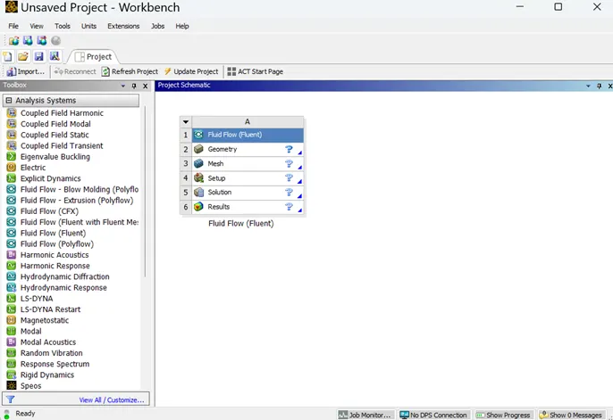
• In Geometry open the spaceclaim for the topology clean-up of the model.

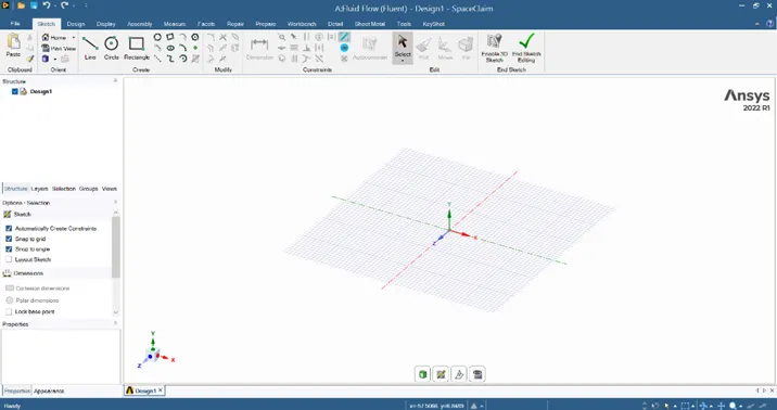
• Import the geometry file of the short mixing tee.

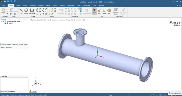
• Suppress the unwanted faces from the geometry for the fluid flow analysis.

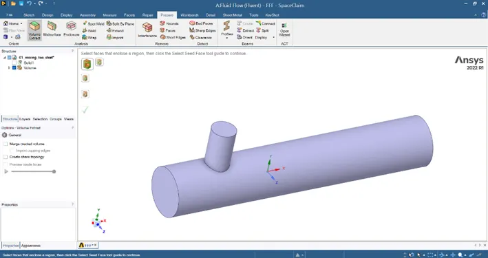
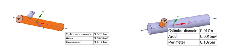
• Measure the diameter of the cold inlet and hot inlet for the future analytical calculation.

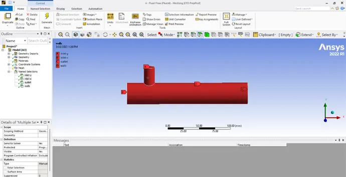
• Close the spaceclaim and go to mesh. Create the named selection to the model.

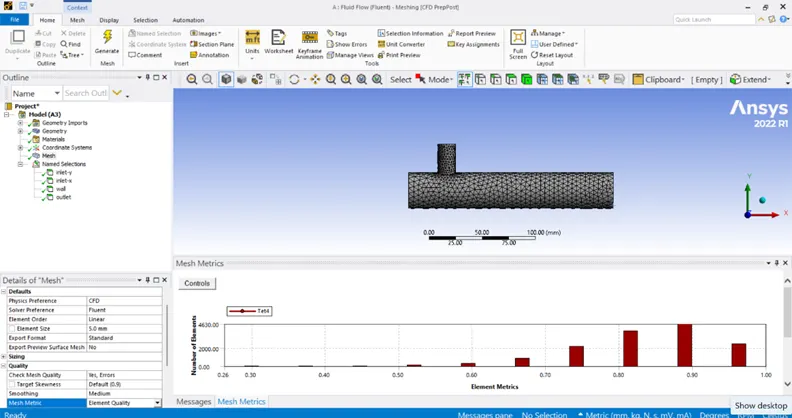
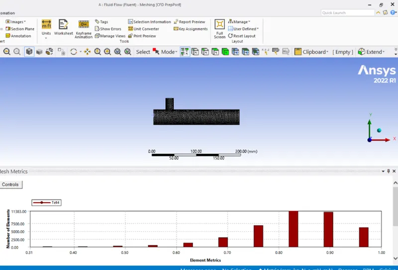
• Generate the mesh and check mesh metric for the quality of the mesh. For the coarse mesh Element metric is 29% and the mesh always should have minimum quality of 5%.

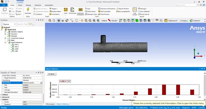
• For the fine mesh we have taken 5mm mesh. check mesh metric for the quality of the mesh. For the fine mesh Element metric is 30%.

• Solving:
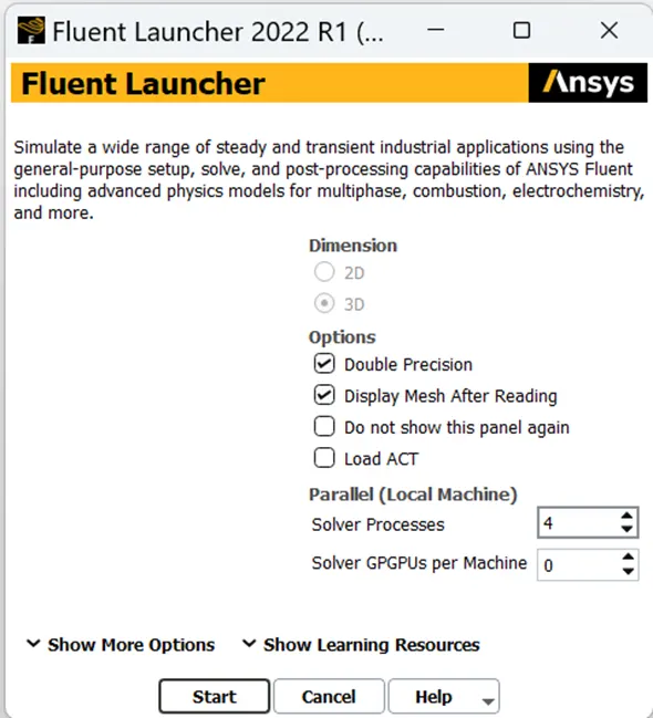
• Open the setup for applying the boundary condition for the fluid flow solution.

Setup	SST K-Omega	K-Epsilon
Solver time	Steady state	Steady state
Solver type	Pressure Based	Pressure Based
Energy Equation	ON	ON
Viscous Model	SST K-Omega	K-Epsilon
Material	Air	Air
Boundary Condition	o Inlet-x Velocity-3m/s Temp-360C o Inlet-y Velocity-6m/s Temp-190C o Outlet Pressure Outlet o Wall No slip wall. Stationary wall	o Inlet-x Velocity-3m/s Temp-360C o Inlet-y Velocity-6m/s Temp-190C o Outlet Pressure Outlet o Wall No slip wall. Stationary wall

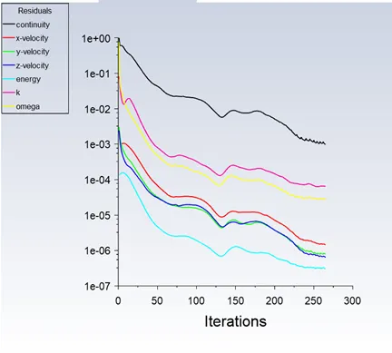
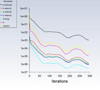
• Scaled residual plots.

SST K-Omega	K-Epsilon

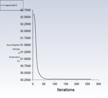
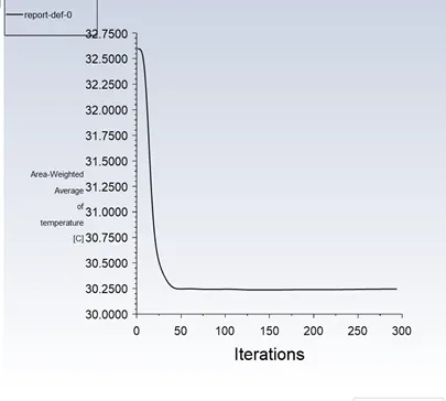
• Area weighted average plots.

SST K-Omega	K-Epsilon

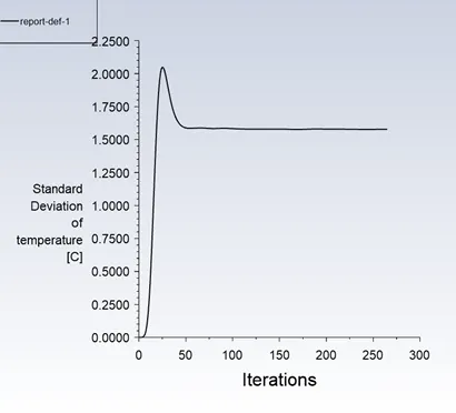
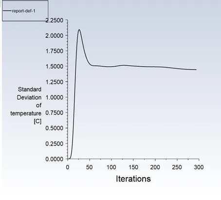
• Standard deviation plots.

SST K-Omega	K-Epsilon

• Post-processing:
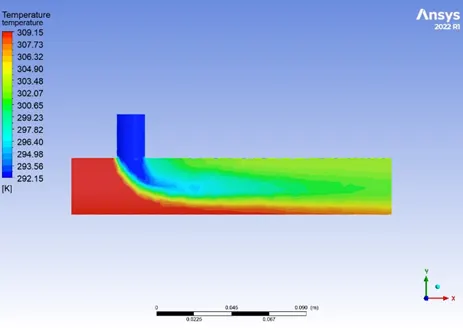
• Temperature contour of the Short Tee for M.R =2

SST K-Omega	K-Epsilon

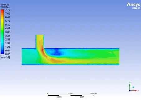
• Velocity contour of the Short Tee for M.R =2

SST K-Omega	K-Epsilon

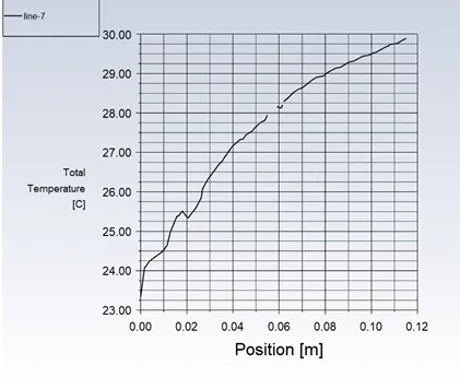
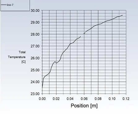
• Temperature line plot across the length

SST K-Omega	K-Epsilon

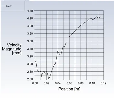
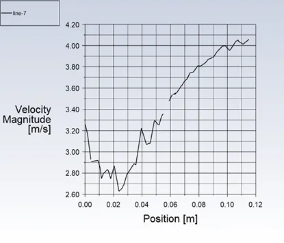
• Velocity line plot across the length

SST K-Omega	K-Epsilon

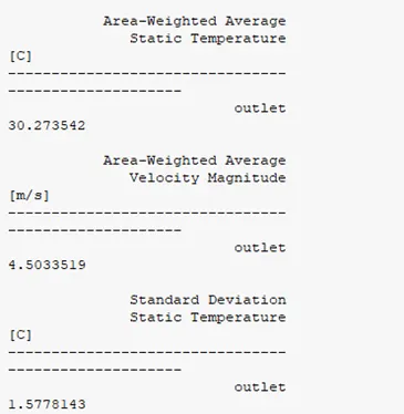
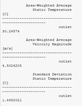
Report Definition:

SST K-Omega	K-Epsilon

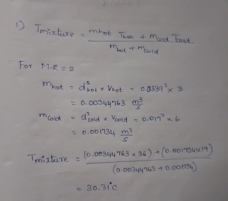
Analytical Solution:

Conclusion for Short Tee M.R =2

The results of the short tee M.R =2 is not having any significant changes using both k-omega sst and k-epsilon model while compared with analytical solution.

• Short Tee for M.R = 4

Pre-processing:

• For this case there is no change in pre-processor. So we have been used same meshed model for the further analysis.
• In this case we only change the setup conditions.

Solving:

• Open the setup for applying the boundary condition for the fluid flow solution.

Setup	SST K-Omega	K-Epsilon
Solver time	Steady state	Steady state
Solver type	Pressure Based	Pressure Based
Energy Equation	ON	ON
Viscous Model	SST K-Omega	K-Epsilon
Material	Air	Air
Boundary Condition	o Inlet-x Velocity-3m/s Temp-360C o Inlet-y Velocity-12m/s Temp-190C o Outlet Pressure Outlet o Wall No slip wall. Stationary wall	o Inlet-x Velocity-3m/s Temp-360C o Inlet-y Velocity-12m/s Temp-190C o Outlet Pressure Outlet o Wall No slip wall. Stationary wall

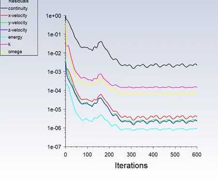
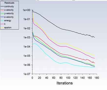
• Scaled residual plots.

SST K-Omega	K-Epsilon

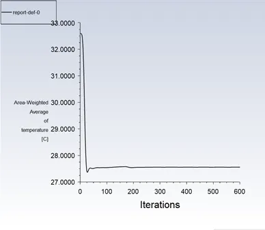
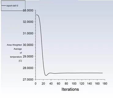
• Area weighted average plots.

SST K-Omega	K-Epsilon

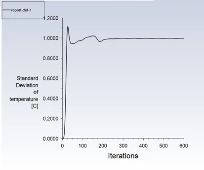
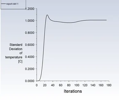
• Standard deviation plots.

SST K-Omega	K-Epsilon

• Post-processing:
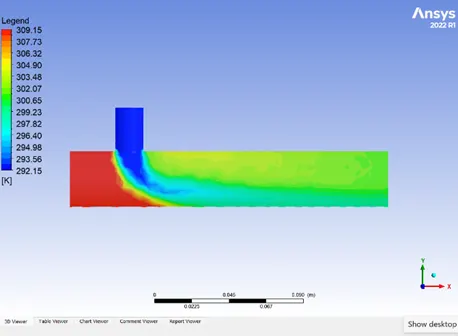
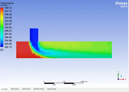
• Temperature contour of the Short Tee for M.R =4

SST K-Omega	K-Epsilon

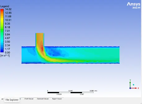
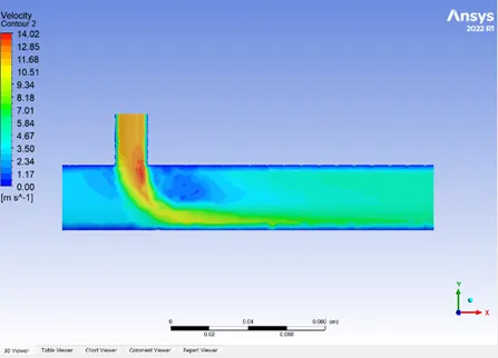
• Velocity contour of the Short Tee for M.R =4

SST K-Omega	K-Epsilon

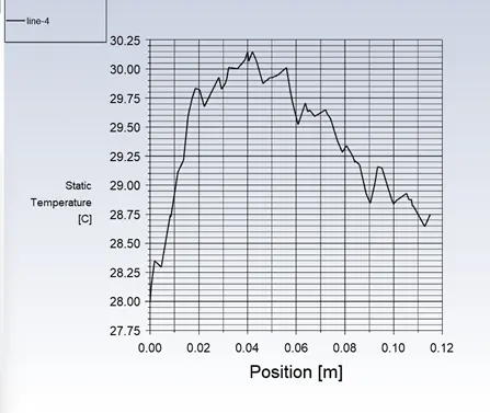
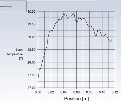
• Temperature line plot across the length

SST K-Omega	K-Epsilon

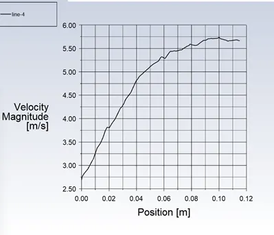
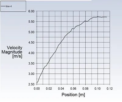
• Velocity line plot across the length

SST K-Omega	K-Epsilon

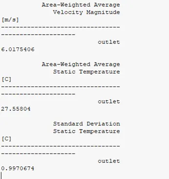
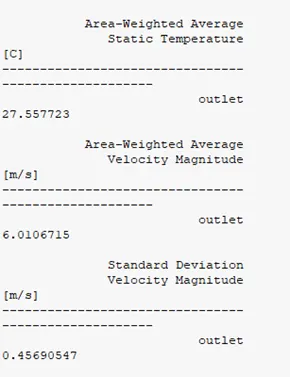
Report Definition:

SST K-Omega	K-Epsilon

Analytical Solution:

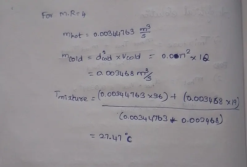
Conclusion for Short Tee M.R =4

The results of the short tee M.R =4 is having significant changes using both k-omega sst and k-epsilon model while compared with analytical solution.

1. From the above cases the k-epsilon having more effectiveness compared to k-omega SST model.
2. Less iteration taken for solution convergence.
3. For upcoming cases we have been using k-epsilon model.

CASE 2: LONG TEE

• Long Tee for M.R = 2

Pre-processing:

• From the analysis system toolbox open the Fluid Flow (Fluent)

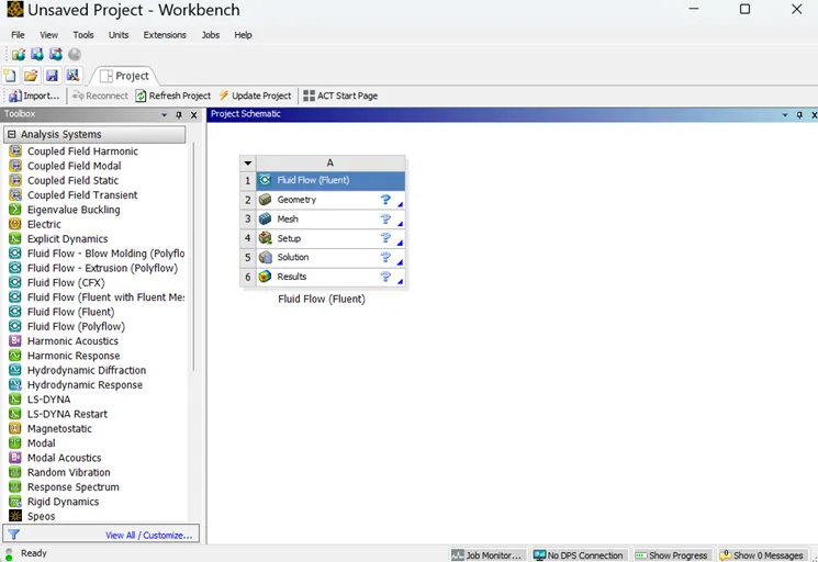
• In Geometry open the spaceclaim for the topology clean-up of the model.

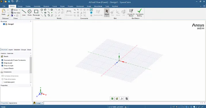
• Import the geometry file of the long mixing tee.

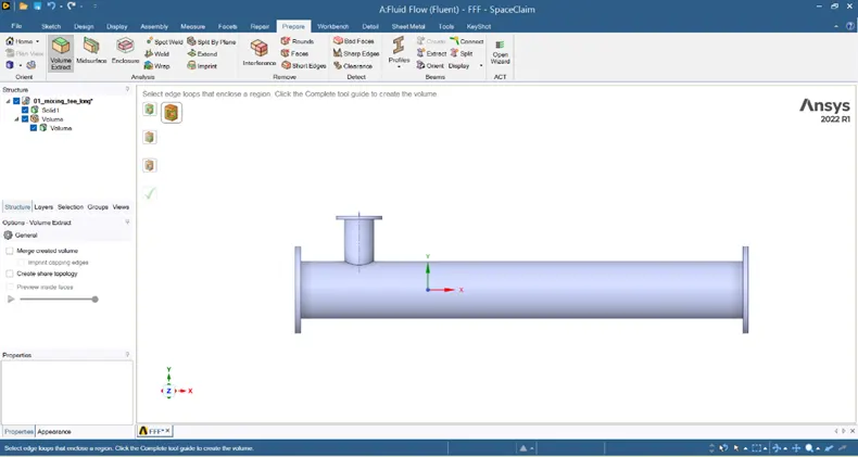
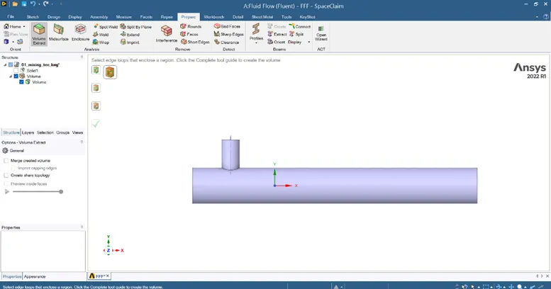
• Suppress the unwanted faces from the geometry for the fluid flow analysis.

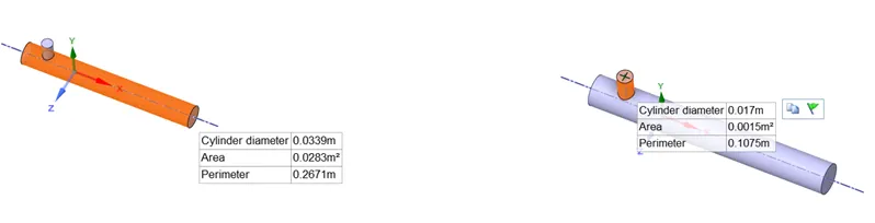
• Measure the diameter of the cold inlet and hot inlet for the future analytical calculation.

• Close the spaceclaim and go to mesh. Create the named selection to the model.

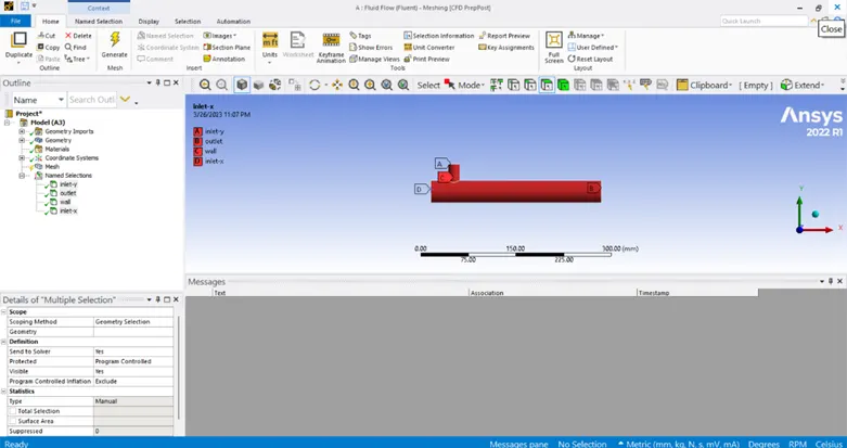
• Generate the mesh and check mesh metric for the quality of the mesh. For the coarse mesh Element metric is 28% and the mesh always should have minimum Element metric of 5%.

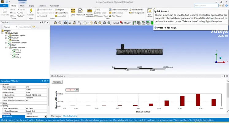
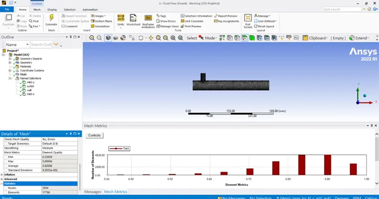
• For the fine mesh we have taken 5mm mesh. check mesh metric for the quality of the mesh. For the fine mesh Element metric is 36%.

• Solving:
• Open the setup for applying the boundary condition for the fluid flow solution.

Setup	K-Epsilon
Solver time	Steady state
Solver type	Pressure Based
Energy Equation	ON
Viscous Model	K-Epsilon
Material	Air
Boundary Condition	o Inlet-x Velocity-3m/s Temp-360C o Inlet-y Velocity-6m/s Temp-190C o Outlet Pressure Outlet o Wall No slip wall. Stationary wall

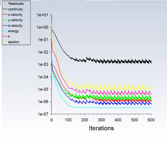
• Scaled residual plots.

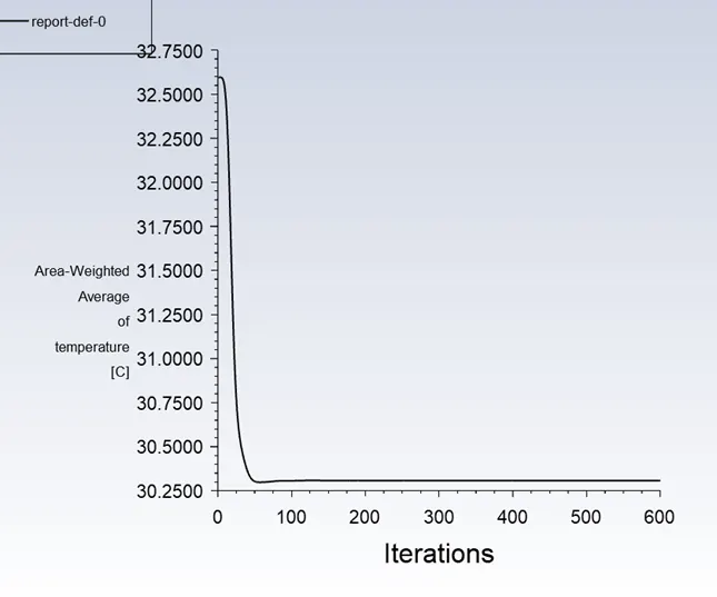
• Area weighted average plots.

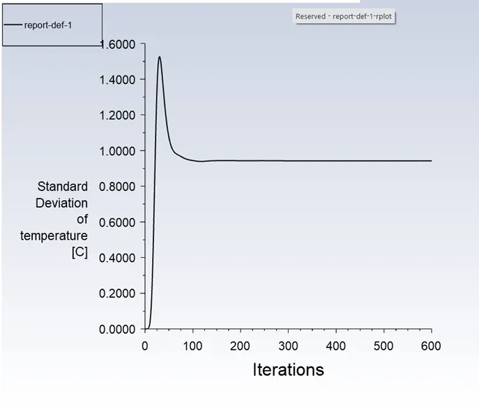
• Standard deviation plots.

• Post-processing:
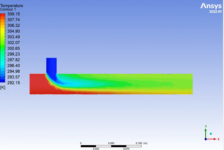
• Temperature contour of the Long Tee for M.R =2

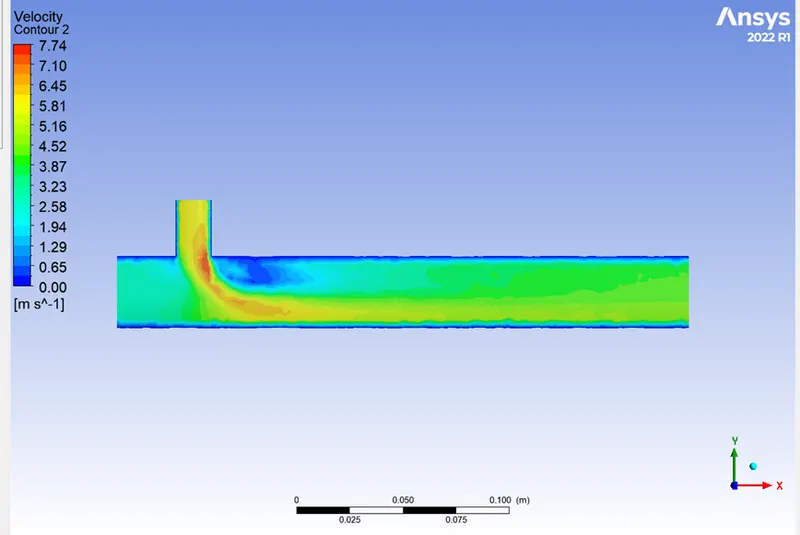
• Velocity contour of the Long Tee for M.R =2

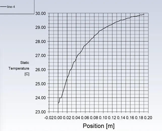
• Temperature line plot across the length

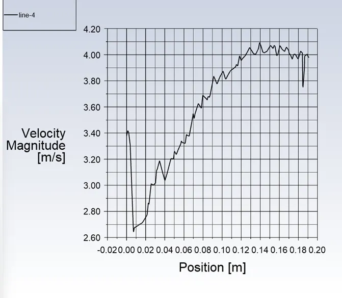
• Velocity line plot across the length

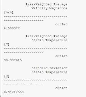
Report Definition:

• Long Tee for M.R = 4

Pre-processing:

• For this case there is no change in pre-processor. So we have been used same meshed model for the further analysis.
• In this case we only change the setup conditions.

Solving:

• Open the setup for applying the boundary condition for the fluid flow solution.

Setup	K-Epsilon
Solver time	Steady state
Solver type	Pressure Based
Energy Equation	ON
Viscous Model	K-Epsilon
Material	Air
Boundary Condition	o Inlet-x Velocity-3m/s Temp-360C o Inlet-y Velocity-12m/s Temp-190C o Outlet Pressure Outlet o Wall No slip wall. Stationary wall

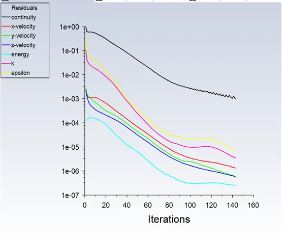
• Scaled residual plots.

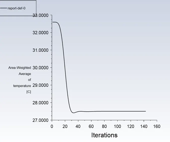
• Area weighted average plots.

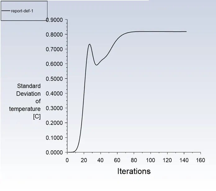
• Standard deviation plots.

• Post-processing:
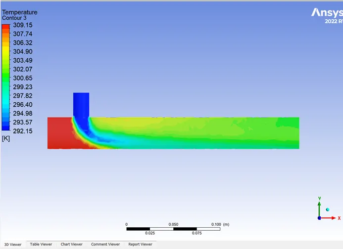
• Temperature contour of the Long Tee for M.R =4

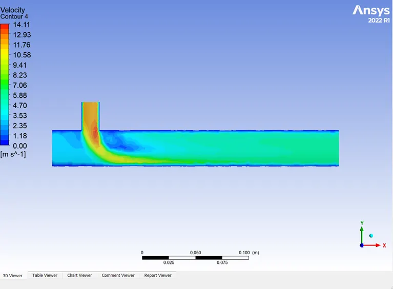
• Velocity contour of the Long Tee for M.R =4

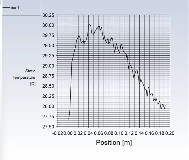
• Temperature line plot across the length

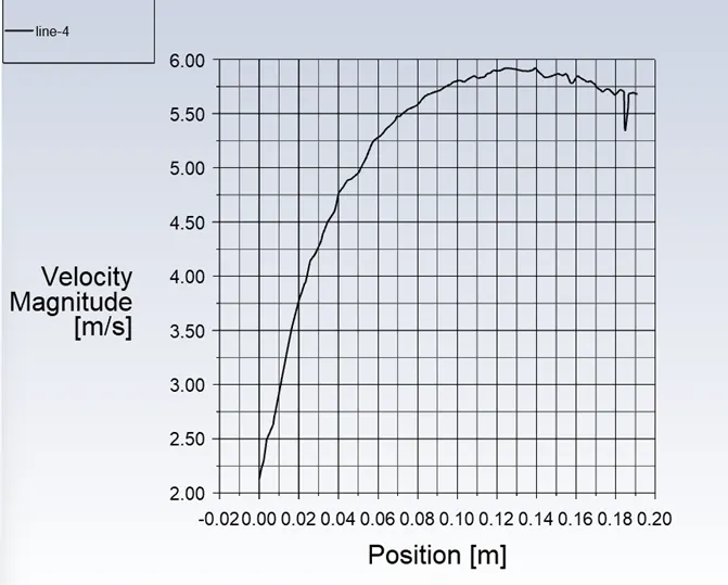
• Velocity line plot across the length

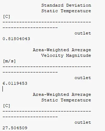
Report Definition:

Conclusion for Long Tee

From the above results, I have concluded that there is no significant change in the result due to increasing the length of the mixing tee. But increasing the momentum ratio it has significant change in result and mixing efficiency is more compared to by increasing the length.

Comparison table:

Model	Momentum Ratio	Number of cell zones	Average outlet temperature (C0)		Number of Iteration for the convergence
			Analytical	Numerical
Short Tee	2	12613	30.24	30.31	294
	4	12613	27.55	27.47	174
Long Tee	2	17796	30.30	30.31	318
	4	17796	27.50	27.47	143

GRID INDEPENDENCE TEST:

• The model which I have chosen for the Grid independence test is the short tee with momentum ratio of 4.

5mm Mesh

• Generate the mesh for 5mm and check mesh metric for the quality of the mesh. For the 5mm mesh Element metric is 36%

3mm Mesh

• Generate the mesh for 3mm and check the mesh metric for the quality of the mesh. For the 3mm mesh Element metric is 37%.

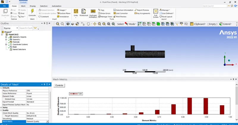
1mm Mesh

• Generate the mesh for 1mm and check the mesh metric for the quality of the mesh. For the 1mm mesh Element metric is 34%.

Mesh Size	Momentum Ratio	Number of cell zones	Average outlet temperature (C0)		Number of Iteration for the convergence
			Analytical	Numerical
5mm	2	12613	30.24	30.31	294
3mm	2	39832	30.29	30.31	340
1mm	2	578113	30.42	30.31	344

From the above table, we have concluded that the mesh size is decreasing to finer and takes more iteration for the convergence of the solution.

Effect of the length and momentum ratio

I have concluded that there is no significant change in the result due to increasing the length of the mixing tee. But increasing the momentum ratio has a significant change in the result and mixing efficiency is more compared to increasing the length.

Conclusion:

From the results, I conclude that there is no need of increasing the length of the mixing while analyzing the mixing efficiency of the mixing tee. By increasing the momentum ratio we can get better results compared to the effect of length.