Week 1- Mixing Tee

REPORT ON MIXING TEE SIMULATION

AIM

To set up steady-state simulations to compare the mixing effectiveness when hot inlet temperature is 36⁰C & the Cold inlet is at 19⁰C.

Use the k-epsilon and k-omega SST model for the first case and based on your judgment use the more suitable model for further cases. Giving the reason for choosing a suitable model is compulsory.

Here it is asked to find it for 2 cases

1. Case 1
   • Short mixing tee with a hot inlet velocity of 3m/s.
   • Momentum ratio of 2, 4.
2. Case 2
   • Long mixing tee with a hot inlet velocity of 3m/s.
   • Momentum ratio of 2, 4.

Momentum ratio = velocity at cold inlet / velocity at hot inlet

Also compare the following values from the 2 cases.

1. Cell count
2. Average outlet temperature
3. Number of iterations for convergence

Also we need to plot

1. Velocity and temperature contour plots on the cut planes along and across the pipe.
2. Velocity and temperature line plots along and across the length of the pipe.

Then we need to perform Mesh independent study for any one case and discuss the effect of length and momentum ratio on results.

THEORY

Mixing Tee is a device which uses specifically engineered internal geometry to mix two fluid streams into one steam, efficiently. In this study we are going to find effectiveness of mixing tee. Hot air and cold air are going to be mixed in mixing tee. They will have different velocities. We will use two different mixing tee distinguished with length and analyse the effect of length on mixing. The main application of this technique is the air conditioning system, where air from the atmosphere along with circulating cold air is mixed with each other to a comforting temperature (say around `24^circ C`) and supplied to the room.

We also use the equation Momentum ratio = velocity at cold inlet / velocity at hot inlet, to calculate the velocity at cold inlet since the velocity at hot inlet is given as 3 m/s and Momentum ratio as 2,4 we calculate velocity for both the ratios.

Since velocity at hot inlet is 3 m/s for Momentum ratio =2 we have velocity at cold inlet = 6 m/s and for ratio = 4 we have velocity at cold inlet = 12 m/s

We also calculate the outlet temperature using the equation `T_(mixture) = (m_(hot)*T_(hot)+m_(cold)*T_(cold))/(m_(hot)+m_(cold))`

For m =2 T_mixture = 30.2 degree celcius

PROCEDURE

The first step is to open Ansys workbench and click and drag the Ansys(Fluent) version from toolbox to the project window which opens the following tool which shows the steps taken for the completion of the simulation process

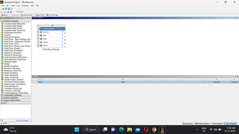
In the above image we can see the steps for carrying out the simulation out of which the first one is the creation of the geometry.Here the firststep is the creation of the geometry and then we do the meshing along with naming the parts of inlets, outlet and walls. Then we move to the set up part where we provide the user defined conditions like boundary conditions For that we double click on the geometry and open it in spaceclaim and first open the short mixing Tee

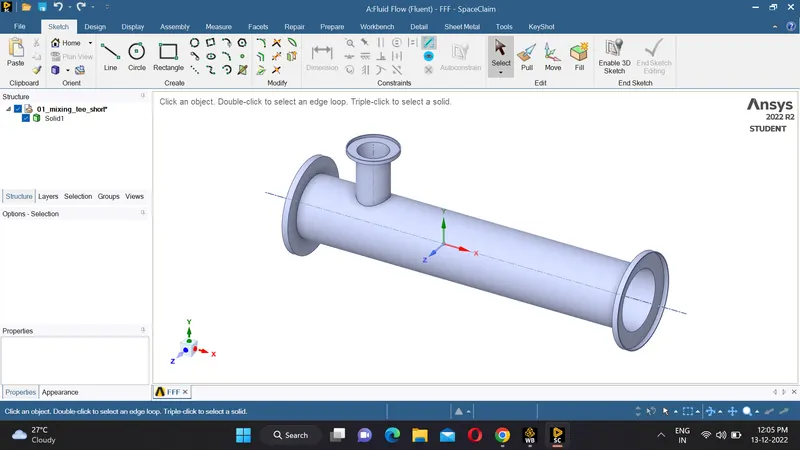
Then we remove the edges which are not required using volume extract tool present inside the prepare file. We remove the edges using the edge extraction tool inside the volume extraction tool, by selecting the volume which we need for the simulation as shown below

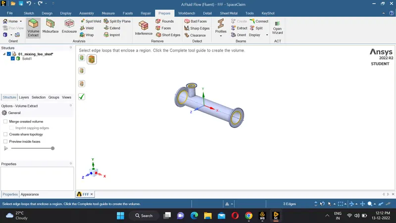
After clicking ok the required volume that is extracted will be as shown below

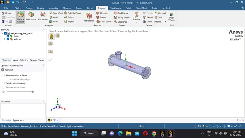
Then we have to remove the solid body since we require only the volume thus we uncheck the solid1 and suppress it for physics. Thus we get the required volume

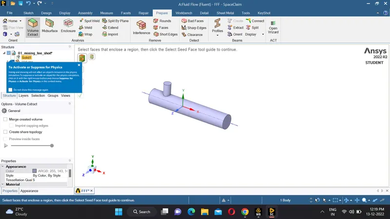
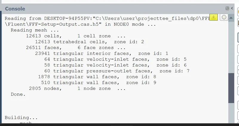
Now we close the spaceclaim which will be automatically saved and then we open mesh and first we name the parts like the two inlets and outlet and walls as inlet-x, inlet-y, outlet , wall1 and wall2

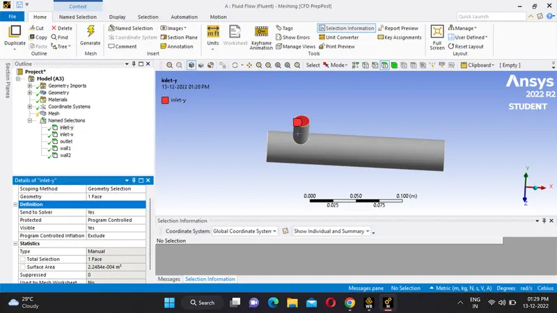
For naming we select a face and press the key 'n' to name the face this is done for all the faces in the similar manner resulting in the named selections as shown in the above image

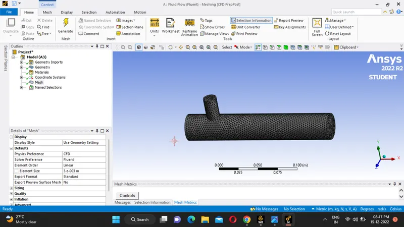
Then we generate the mesh, it will generate mesh according to some predefined criteria. Element size can be selected but it is going to affect simulation time. Section plane can be created to see inner portion of geometry.

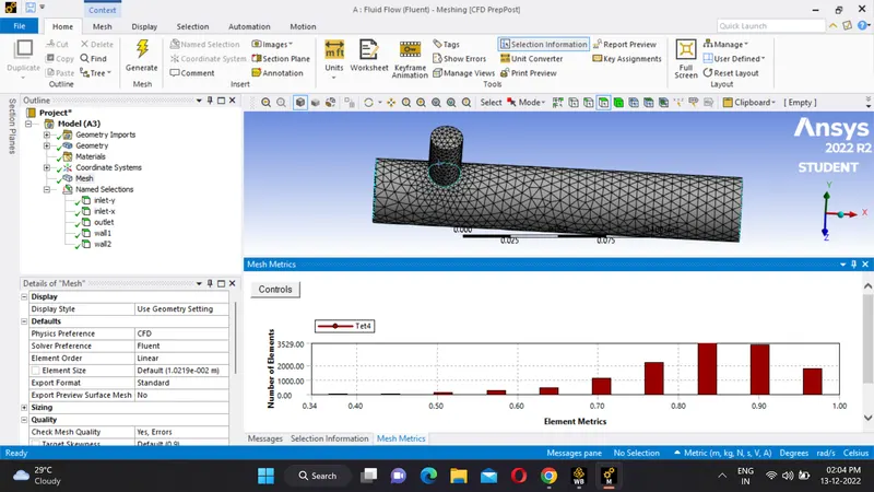
In the above image we also have a graph of element metrices against number of elements which shows the element quality which should be a minimum of 5 percent here the minimun quality is 34 percent thus the meshing is of good quality to continue.

Then we exit mesh and open set up where we give the boundary conditions and all the necessary input conditions

Then we give the given type of solver we use that is pressure based steady state solver with the absolute velocity formulation as shown below

We use Pressure based solver because we have the Mach number less than 0.3 for fluids with Mach no less than o.3 we use Pressure based solver, if Mach no is greater than 0.3 then we use Density based Solver

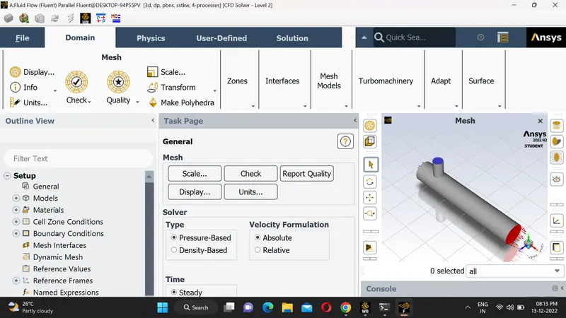
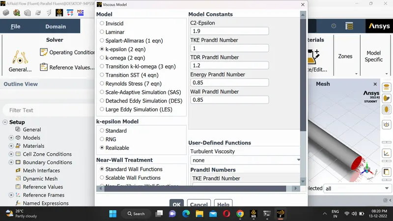
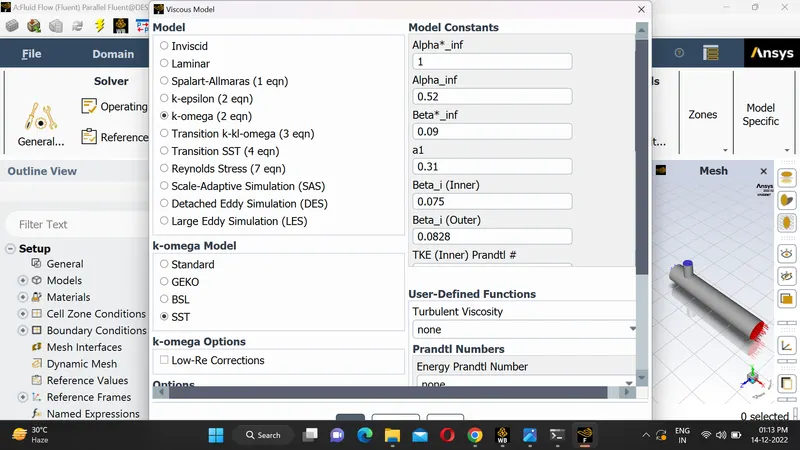
Now we check the mesh and then provide the necessary details using the physics tool bar and then we provide the k epsilon model at first with the realizable model as shown below

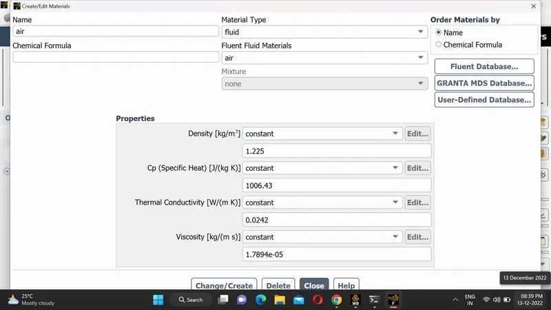
Then we check the materials, since the material is air there is no changes required in the material selection part

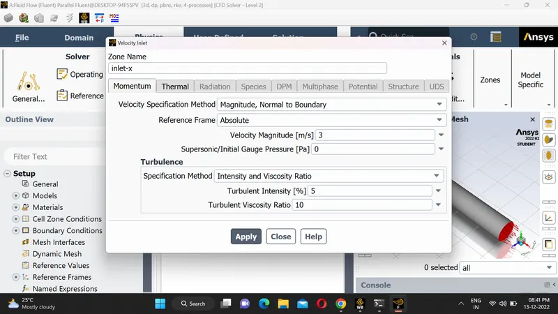
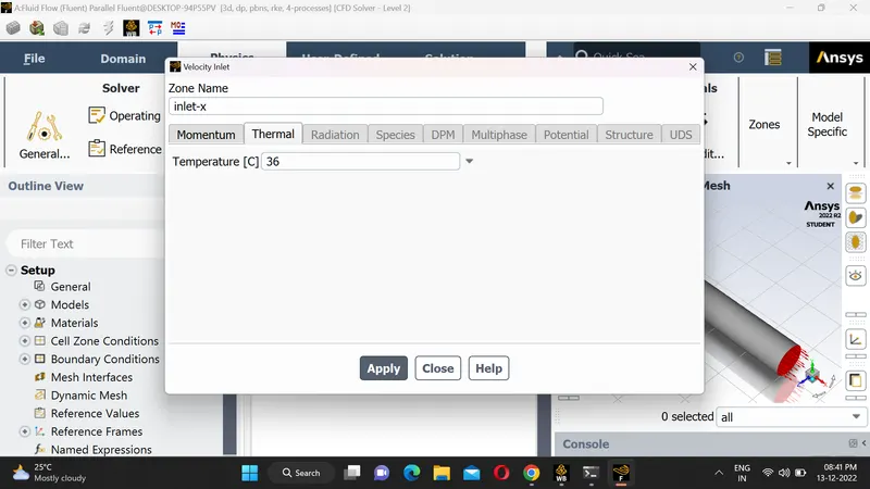
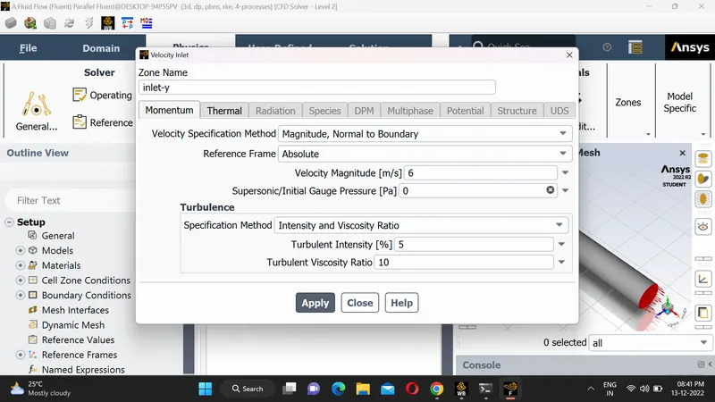
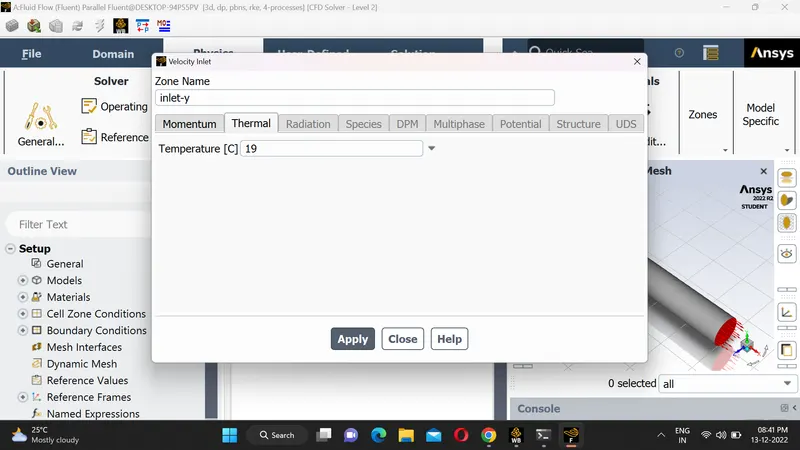
then we give the boundary conditions that are provided in the question i.e hot inlet temperature is 36⁰C & the Cold inlet is at 19⁰C and we are also given with the velocity at hot inlet and also we calculate the velocity at cold inlet using the momentum ratio and also provide it as the boundary condition at cold inlet

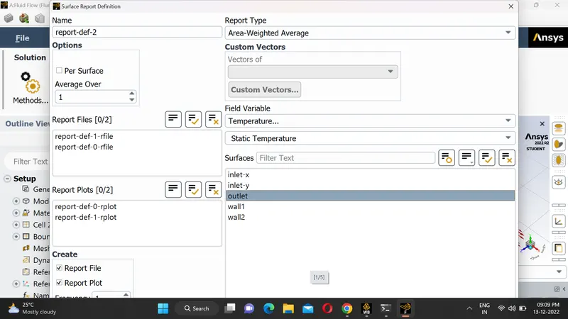
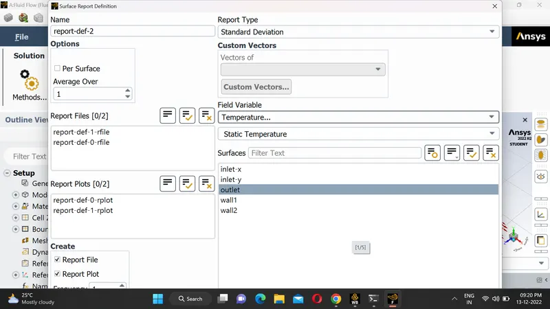
We want to generate temperature report of outlet and we want standard deviation of temperature also. Go to solutions tab and select definition and select area weighted average. In the opened menu select temperature as field variable. Similarly select standard deviation in definitions menu.

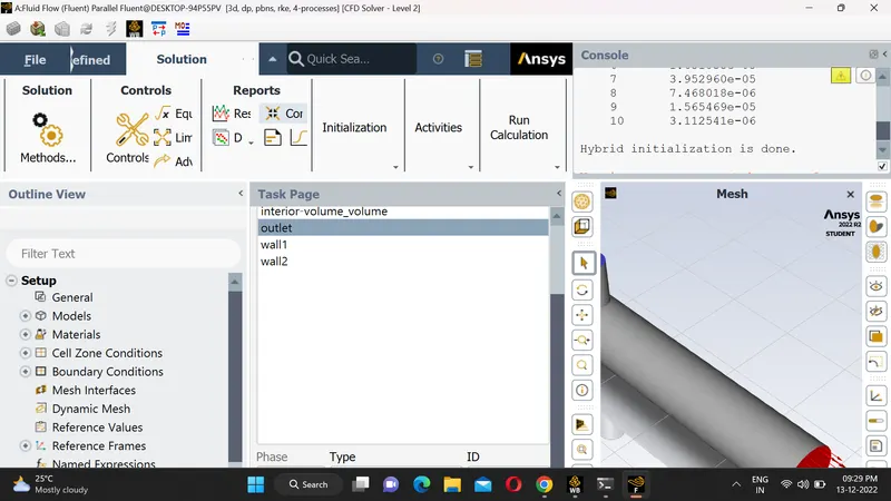
Now we initialise the simulation and then we give the number of iterations as 150 and Change the number of iterations to 250 and click on calculate. If solution is not converged, then iterations can be increased.

Exit setup and double click on result to open CFD post. Check boxes to see walls and other parts. Click on walls and go to render set transparency of 0.78 to inside of wall. Colour can also be changed to white for clear visibility.

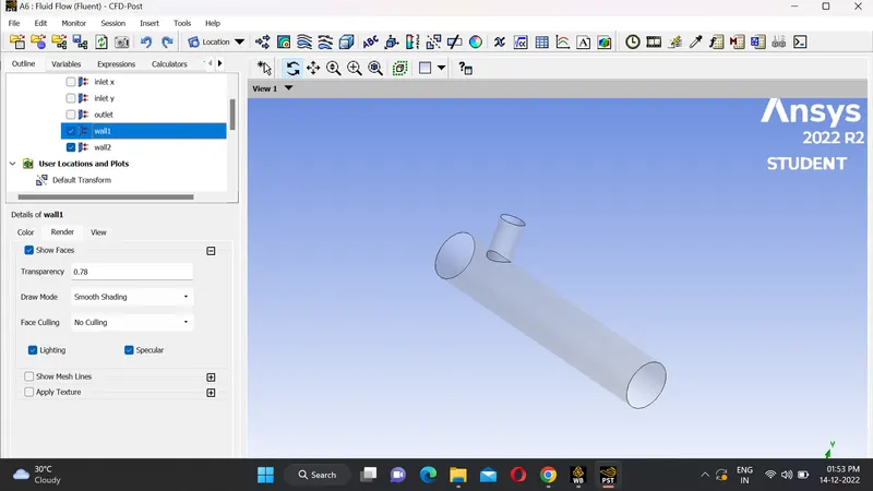
Now insert a XY plane in wall by clicking on plane in location option of insert.

Then we go to colour of plane and change it by variable choose option temperature. Similarly, velocity contours can be created by just changing variable as velocity.

Right click on plane which we created and select streamline. Go to appearance and select temperature to see plot line on plane. Similar procedure can be repeated for velocity plot line.

Then we post process the simulation that is being carried out and check whether the accurate converging has achieved or not. The same procedure is carried out for`k-omega` model with SST as model and all the required plots are noted down.

RESULTS

Comparing the following values from the 2 cases.

Moment Ratio	Cell Count 2 4	Average Outlet Temperature 2 4	Number of Iterations for Convergence 2 4
Case 1: Short Tee	12613 12613	30.226 27.479	150 150
Case 2: Long Tee	15530 15530	30.386 27.552	150 130

From above results we can say that outlet temperature is independent of length of the mixing tee.

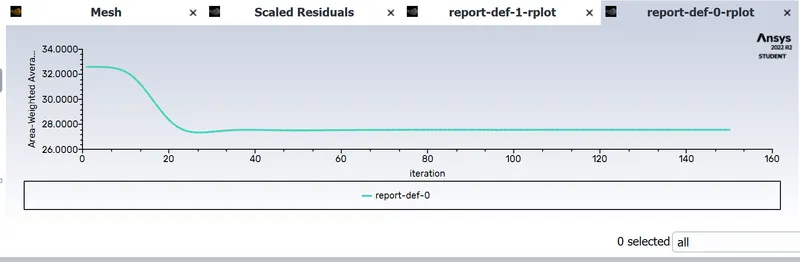
Momentum ratio effects the outlet temperature. By increasing the momentum ratio outlet temperature is dropping.

From above validation of numerical and analytical values we can say that numerical simulation values are matching with analytical values.

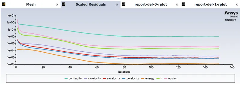
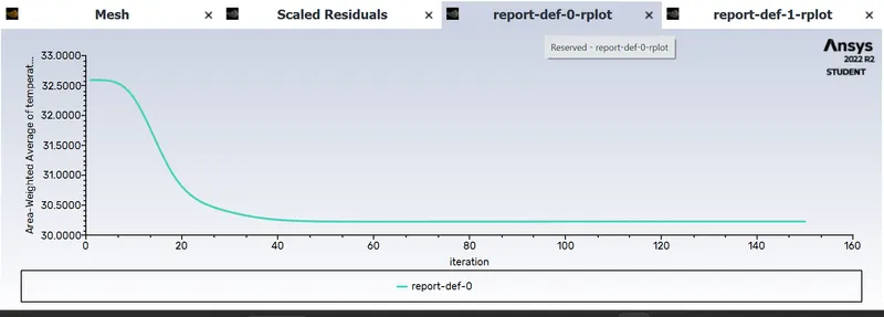
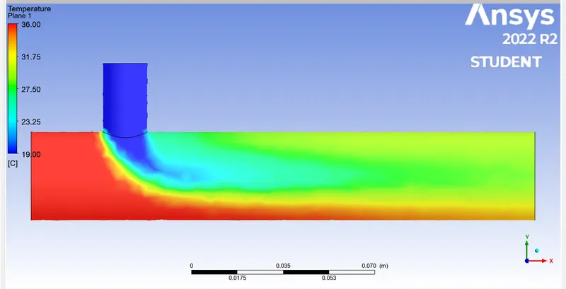
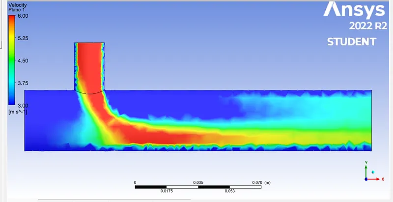
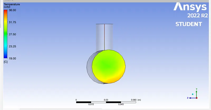
Case 1: Short Mixing Tee with Momentum ratio =2, cold inlet temperature = 19 degree celcius, hot inlet temperature = 36 degree celcius, cold inlet velocity = 6 m/s, hot inlet velocity = 3 m/s , mixture temperature = 30.2 degree celcius, Number of iterations = 150

Scaled Residuals

Area Weighted Average of temperature vs Iterations

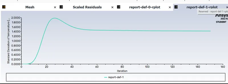
Standard Deviation

Temperatue contour plot along the pipe:

Velocity contour plot along the pipe:

Temperatue contour plot across the pipe:

Velocity contour plot across the pipe:

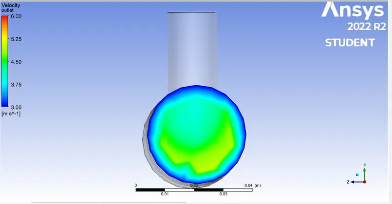
In the post processing part we can see that there is diffused thus we increase the number of iterations

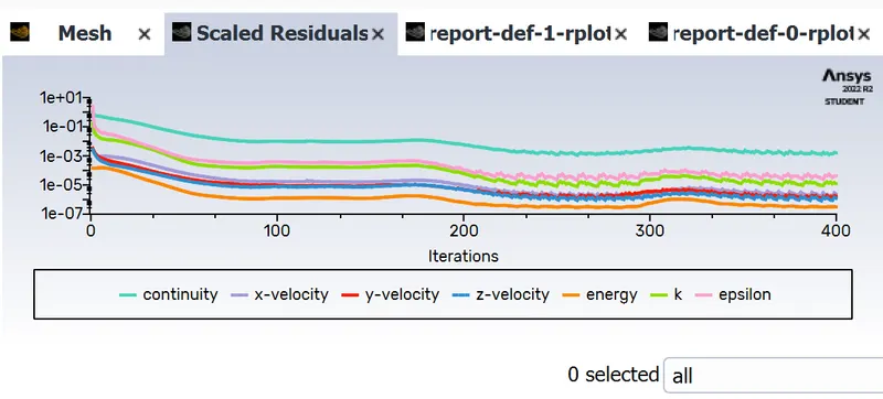
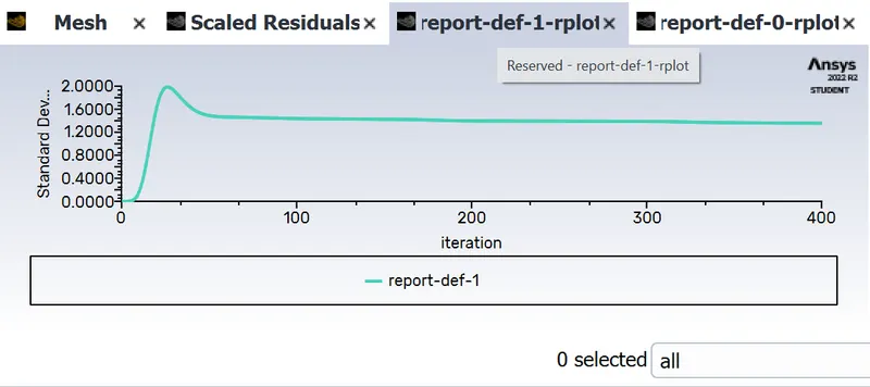
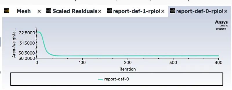
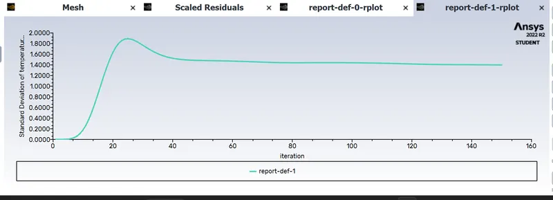
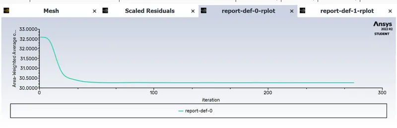
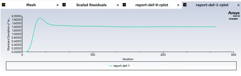
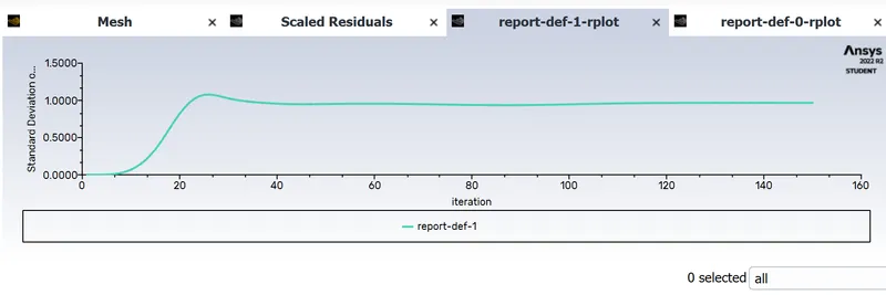
In the above plots we get a graph which is converging at a standard deviation of 1.4, but we still increase the number of iterations to 400 to check whether the values are converged in the right sense.

Scaled Residuals

Standard Deviation

Area Weighted Average of temperature vs Iterations

Temperatue contour plot along the pipe:

Velocity contour plot along the pipe:

Temperature contour plot across the pipe:

Velocity contour plot across the pipe:

Case 1: Short Mixing Tee with Momentum ratio =2, cold inlet temperature = 19 degree celcius, hot inlet temperature = 36 degree celcius, cold inlet velocity = 6 m/s, hot inlet velocity = 3 m/s , mixture temperature = 30.2 degree celcius, Number of iterations = 150 with k-omega as the model type and type SST

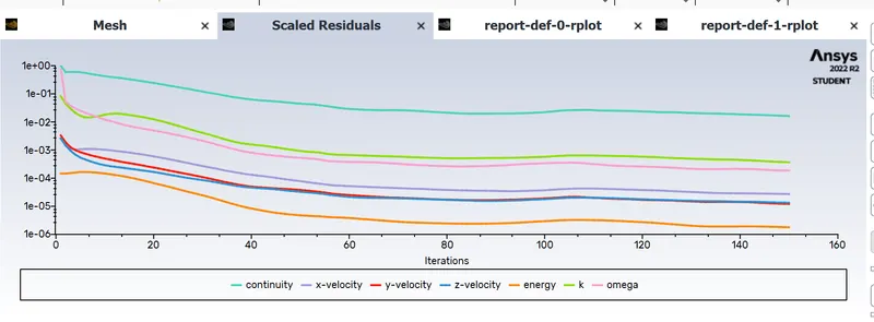
Scaled Residuals

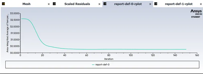
Area Weighted Average of temperature vs Iterations

Standard Deviation

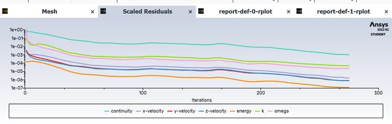
For number of iteration = 400 we have

Scaled Residuals

Area Weighted Average of temperature vs Iterations

Standard Deviation

Temperatue contour plot along the pipe:

Velocity contour plot along the pipe:

Temperature contour plot across the pipe:

Velocity contour plot across the pipe:

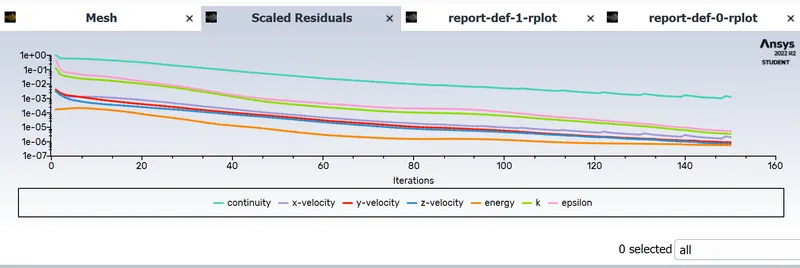
From the residual graph it seems like the solution converge quickly at k-omega model as compared to k epsilon model

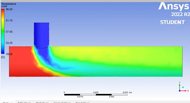
Short Mixing Tee with Momentum ratio = 4, cold inlet temperature = 19 degree celcius, hot inlet temperature = 36 degree celcius, cold inlet velocity = 12 m/s, hot inlet velocity = 3 m/s , mixture temperature = 30.2 degree celcius, Number of iterations = 150 with k-epsilon model.

Scaled Residuals

Area Weighted Average of temperature vs Iterations

Standard Deviation

Temperatue contour plot along the pipe:

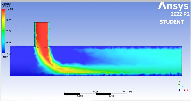
Velocity contour plot along the pipe:

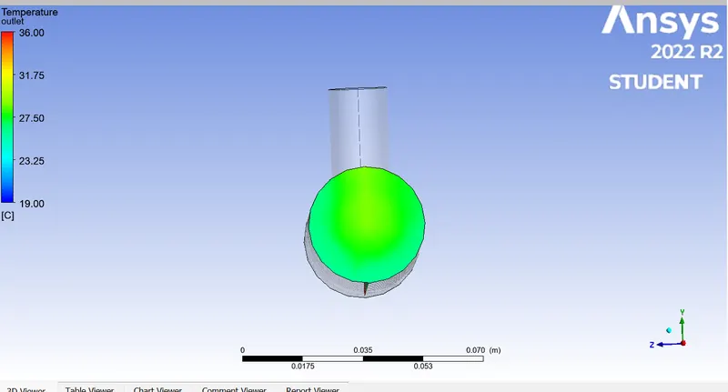
Temperature contour plot across the pipe:

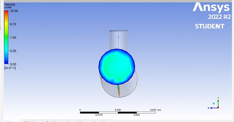
Velocity contour plot across the pipe:

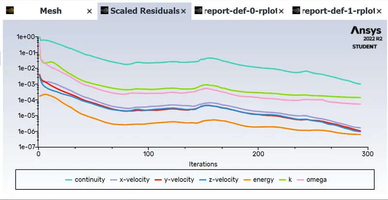
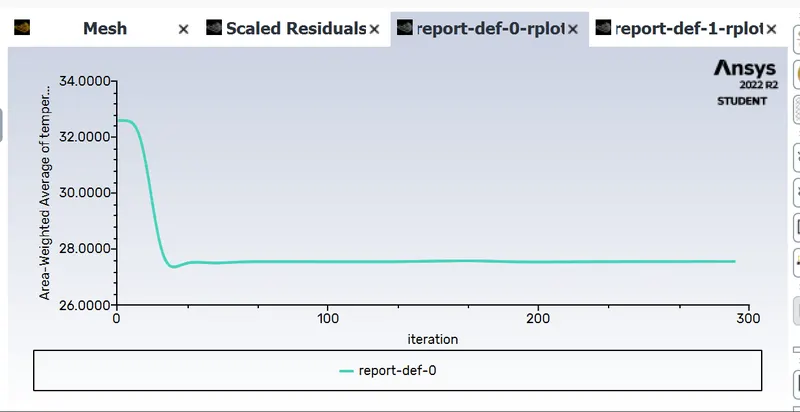
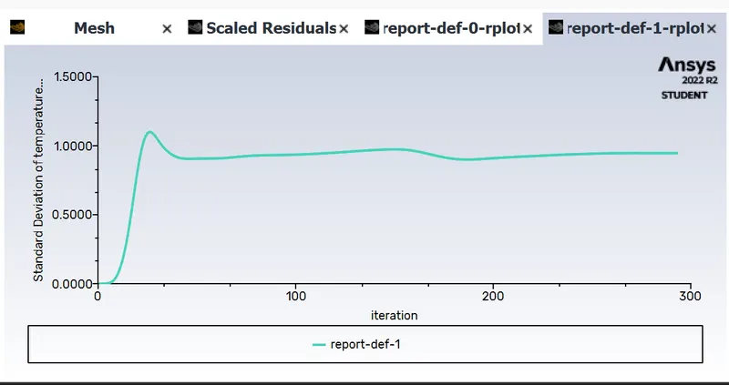
Short Mixing Tee with Momentum ratio = 4, cold inlet temperature = 19 degree celcius, hot inlet temperature = 36 degree celcius, cold inlet velocity = 12 m/s, hot inlet velocity = 3 m/s , mixture temperature = 30.2 degree celcius, Number of iterations = 300 with k-omega model SST

Scaled Residuals

Area Weighted Average of temperature vs Iterations

Standard Deviation

Temperatue contour plot along the pipe:

Velocity contour plot along the pipe:

Temperature contour plot across the pipe:

Velocity contour plot across the pipe:

From the plots and simulation we can conclude that as momentum ratio increases the mixture temperature reduces drastically i.e. for Momentum ratio = 2 Mixture Temperature was 30.2 degree celcius whereas for Momentum ratio 4 the Mixture Temperature became 27.4 degree celcius

At Momentum ratio =2 At Momentum ratio =4

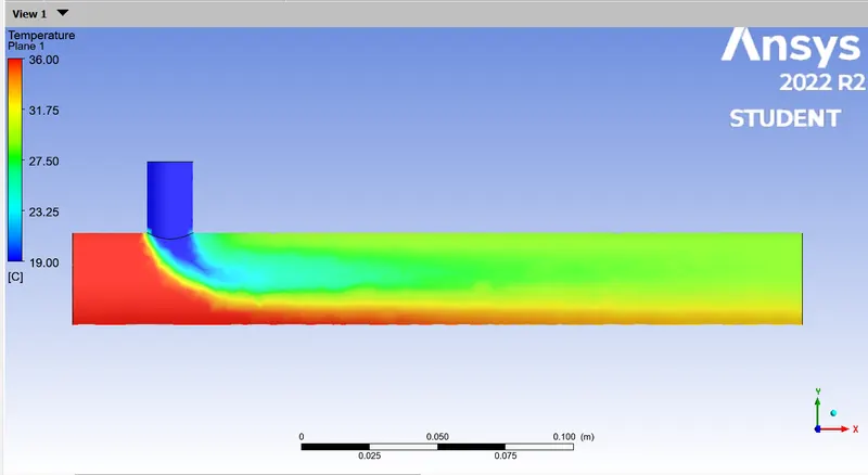
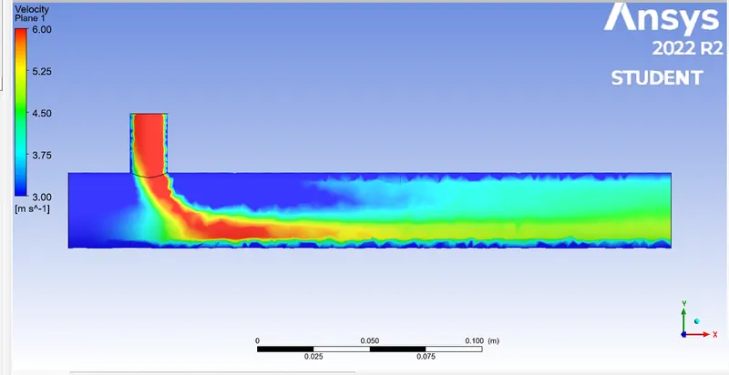
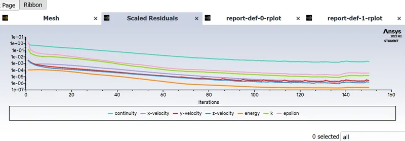
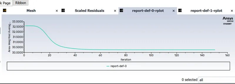
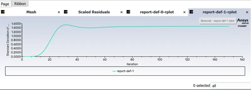
Case 2: Long Mixing Tee with Momentum ratio =2, cold inlet temperature = 19 degree celcius, hot inlet temperature = 36 degree celcius, cold inlet velocity = 6 m/s, hot inlet velocity = 3 m/s , mixture temperature = 30.2 degree celcius, Number of iterations = 150

In the Long Mixing Tee the procedure is same as the Short Mixing Tee, we do all the steps and then we do the post processing. Here we take the long mixing tee and simulate it using the k-epsilon model

Here I took K-epsilon Model for Long Tee model since we have to calculate the Tempearture and Velocity away from the wall.

Temperatue contour plot along the pipe:

Velocity contour plot along the pipe:

Temperature contour plot across the pipe:

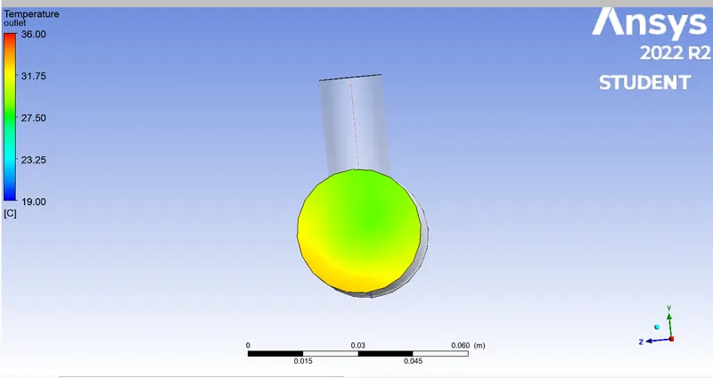
Velocity contour plot across the pipe:

Scaled Residuals

Area Weighted Average of temperature vs Iterations

Standard Deviation

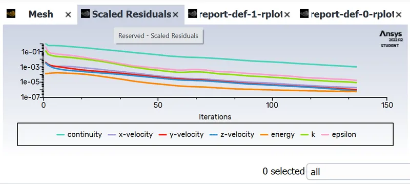
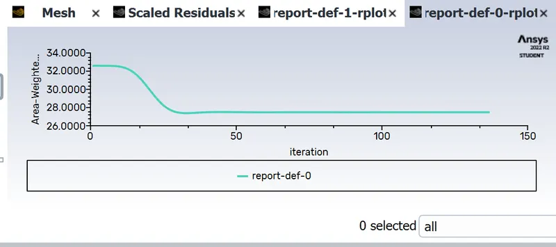
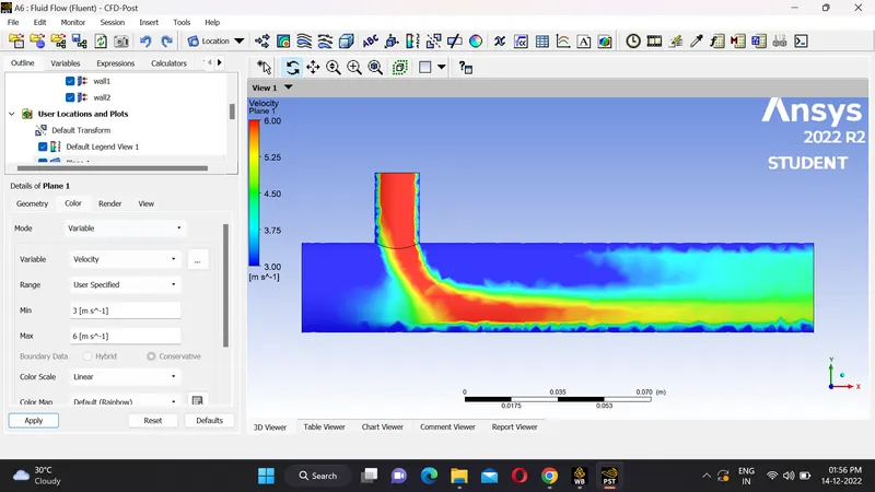
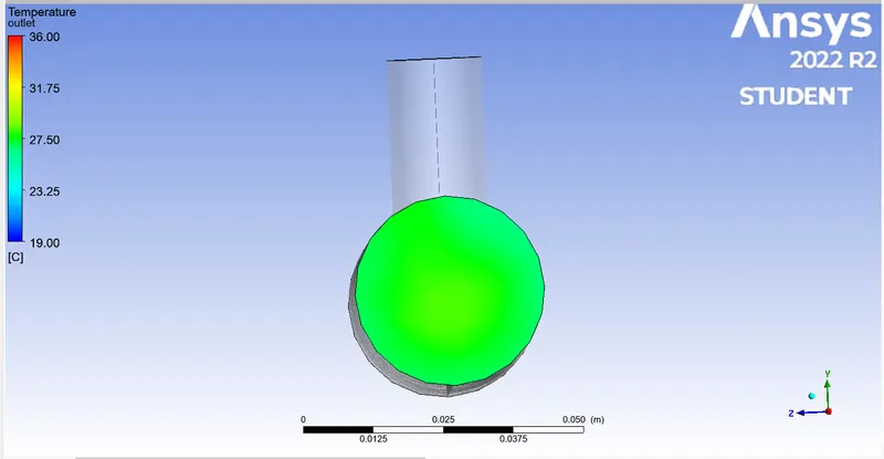
Case 2: Long Mixing Tee with Momentum ratio =4, cold inlet temperature = 19 degree celcius, hot inlet temperature = 36 degree celcius, cold inlet velocity = 12 m/s, hot inlet velocity = 3 m/s , mixture temperature = 30.2 degree celcius, Number of iterations = 150

Scaled Residuals

Area Weighted Average of temperature vs Iterations

Standard Deviation

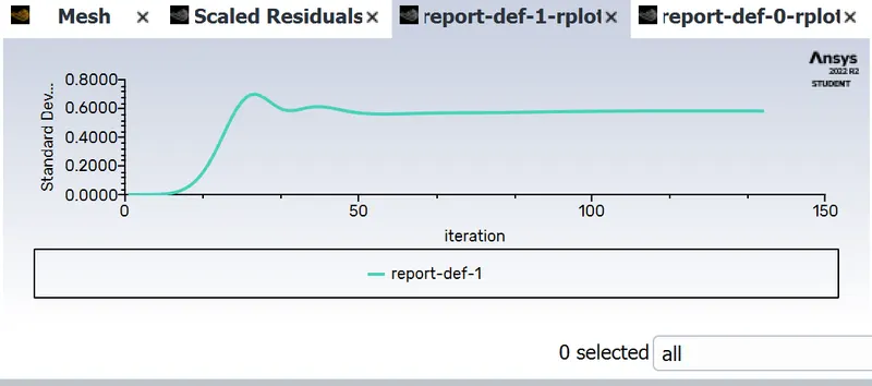
In the above plot the solution converged at 130 iterations that is why even though we gave 150 iterations the plot is terminated at 130 iterations

Temperatue contour plot along the pipe:

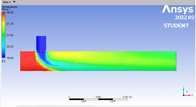
Velocity contour plot along the pipe:

Temperature contour plot across the pipe:

Velocity contour plot across the pipe:

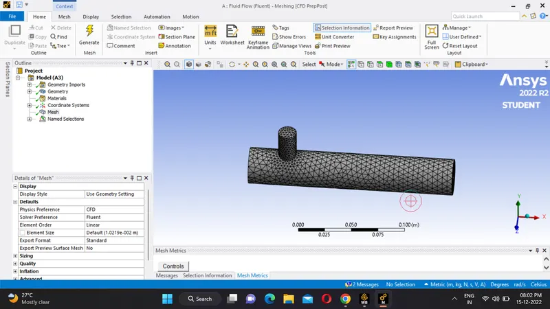
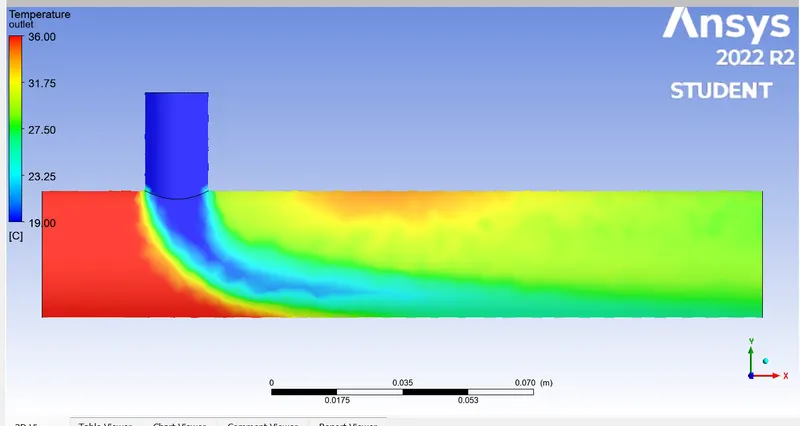
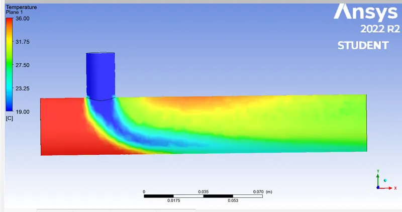
Now let us do the Mesh Independent study for the Short Tee

Initial Case:0.0102

Element Size 0.004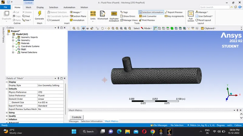

Element Size 0.003

Mesh Size	No. of Cells	Average Temperature
Initial	12613	27.5
0.004	22296	27.586
0.003	40039	26.6309

The above Table shows us that as we decrease the element size the number of cells discretized will increase which results in more accurate value for convergence will be generated.Also from above table we can say that our mesh is independent that means there is no large changes in outlet temperature by increasing the number of elements.

CONCLUSION

After Completing the study we can conclude that as Momentum Ratio increases Average Mixture Temperature decreases and as the outlet temperature is independent of length of the mixing tee. Only advantage is that for Long Mixing Tee the fluids mix more uniformly as compared to the short because the fluid has to travel more length in the mixed state compared to Short Mixing Tee