Week 1- Mixing Tee

Aim: TO analyse the effect of mixing two fluids of various temperature and velocity in a T-pipe using ANSYS.

Introduction: Use ANSYS to prepare a geometry for volumetric meshing and conduct flow analysis on the given geometries. Here k-epsilon and k-omega SST model are used to analyse the mixing of fluids in the T. By analysing the properties of the outlet fluid, we can predict the effectiveness of mixing two gases and thus predict the required velocity and temperature of fluid used in the mixing to achieve the desired output. This is similar to the cooling using air conditioners and heaters.

Solving and modelling: The processes involved in the analysis are Pre-processing, solving and post- processing

In the pre-processing the model is prepared for meshing. After that the required equations for solution are introduced and solving of the equation is done. then the post processing of the solution is done.

In this experiment the hot air is mixed with cold air at different velocities in a short T-joint and in a long T-joint. the outlet air properties are studied using ANSYS. For this we are conducting internal flow analysis of air inside the T.

The T is initially prepared for meshing, for that the internal volume is extracted and then volumetric meshing of the internal volume is done. The mesh used is refined mesh so as to get more accurate results.

After the meshing is complete, then the air properties are given at inlets and the boundary conditions are defined. After the setting of boundary condition, the volume property and outlet property is defined. then the equation for solving the analysis is selected. After entering all variables Iteration is run and results are studied. double precision is used in order to increase the result efficiency. also various graphs of temperature and velocity of outlet air is plotted to understand the outlet air properties such as area weighted average temperature, are weighted average velocity and standard deviation graphs of velocity and temperature.

with iteration required properties are plotted and the solution is analysed.

The solution is found using 2 solvers, K-epsilon and K-omega SST. The iteration result and convergence of both are studied and the best is used for the analysis in the long T.

after that the properties f gas along the cross-section of the T is plotted and analysed. A new plane is inserted inside the T in order to analyse the air properties inside the T.

Pre-processor and Solver: while using ANSYS to analyse the mixing of air in joint the tools used are, Ansys workbench, space claim, mesh, Fluent and solution.

ANSYS workbench is used to initialise the work in ANSYS, to select the type of analysis system and the flow procedure in ANSYS. Here we are using ANSYS Fluid Flow(fluent) for the analysis.

The project schematic gives the current status of the whole process and the flow of the process and the next steps in the analysis.

• Pre-processing

ANSYS Space claim is used to prepare the geometry for pre-processing. In ANSYs Space claim the internal volume of the T is extracted. Volume extract tool in Prepare is used for the internal volume extraction. The volume is selected using the edges option in the volume extract tool. after extracting the internal volume, the solid body is hidden and excluded from further analysis.

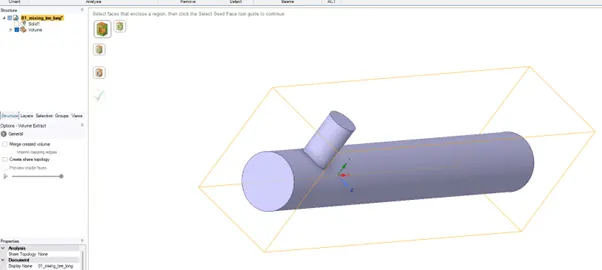
The extracted volume is then meshed using the ANSYS mesh.

ANSYS mesh is opened using the mesh in workbench project flow. Inlets of the T in the X and Y axis are named on the respective faces as inlet-x and inlet-y, outlet as outlet and walls as walls. Naming the faces in the mesh menu the size of mesh is set as .0015mm and then the T is meshed.

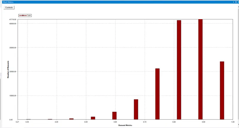
the quality of mesh is checked using the mesh quality > mesh metric > element quality

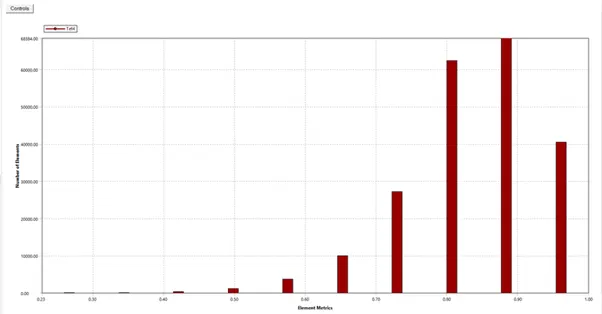
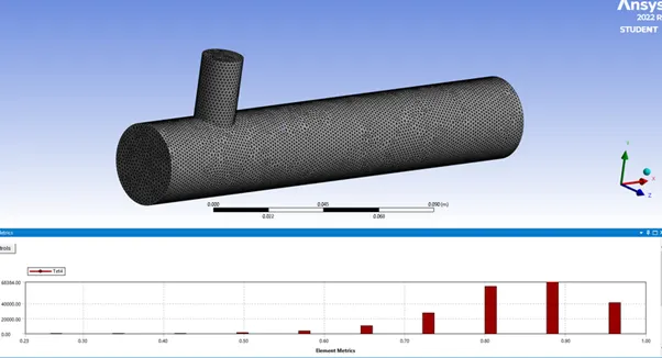
after mesh generation the pre-processing is complete and then proceed to solving.

• Solving

in solving first, we need to set the incoming air properties and the required boundary, inlet and outlet conditions as well as the solver method.

for that Fluent CFD solver is used.

in domain the unit of temperature is set to degree Celsius and the mesh is checked for any errors. then in Physics menu in general solver type is set to Pressure based, velocity formulation is set to absolute and time to steady. energy equation is also implemented.

initially the viscous model is set to K-epsilon realizable model with standard wall functions.

material is created as air. and in cell zones material name is set to air and boundaries are defined

inlet-x air velocity as 3m/s and temperature as 36c and in inlet-y 6m/s and temperature 19c. outlet gauge pressure is set to zero and outlet type as pressure outlet.

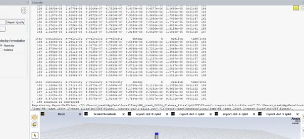
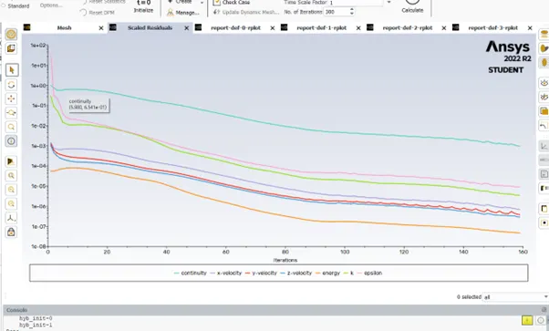
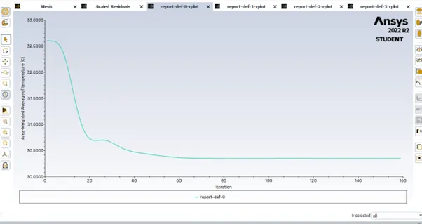
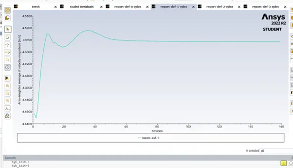
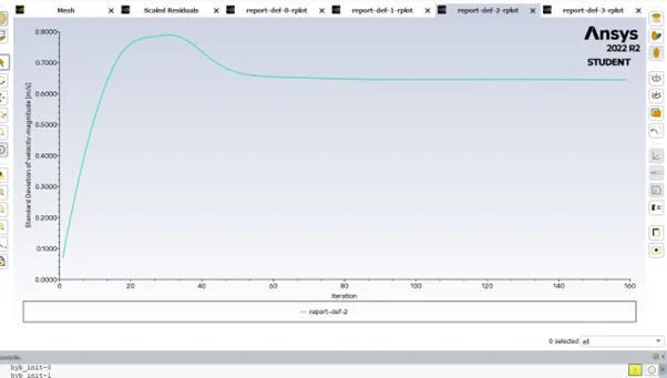
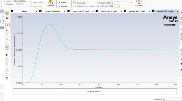
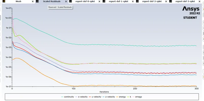
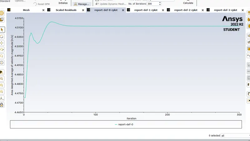
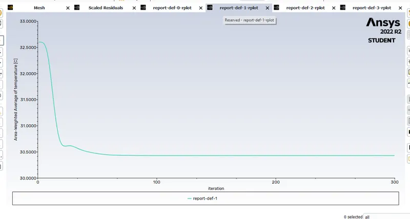
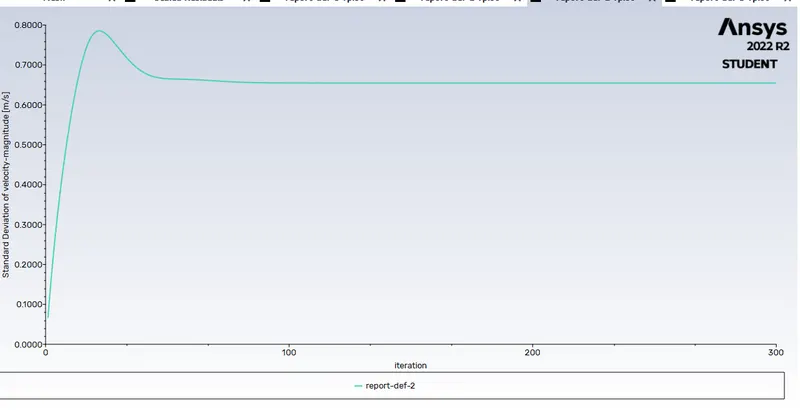
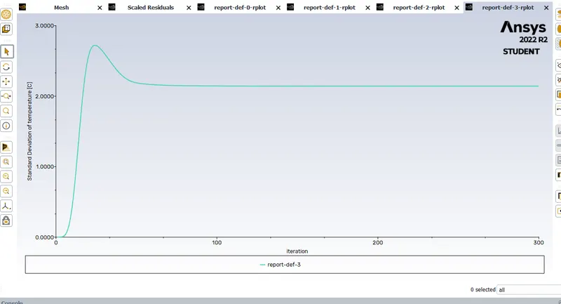
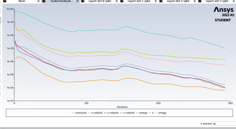
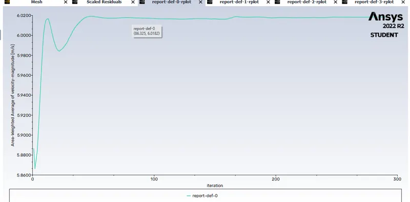
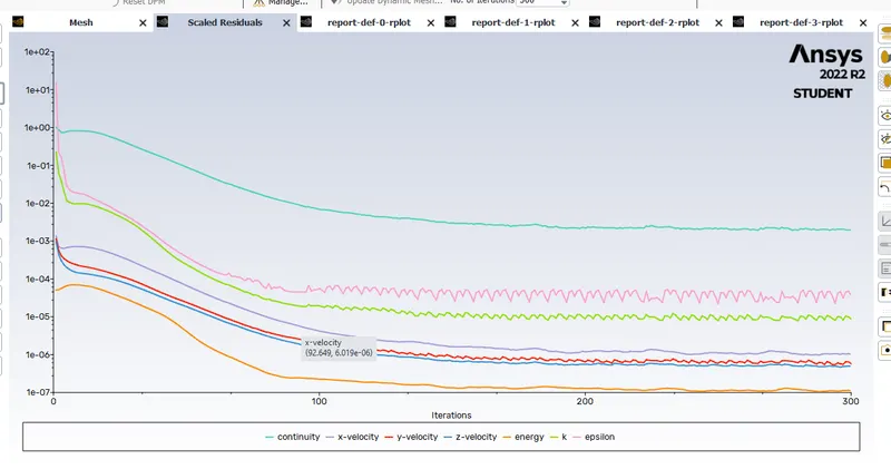
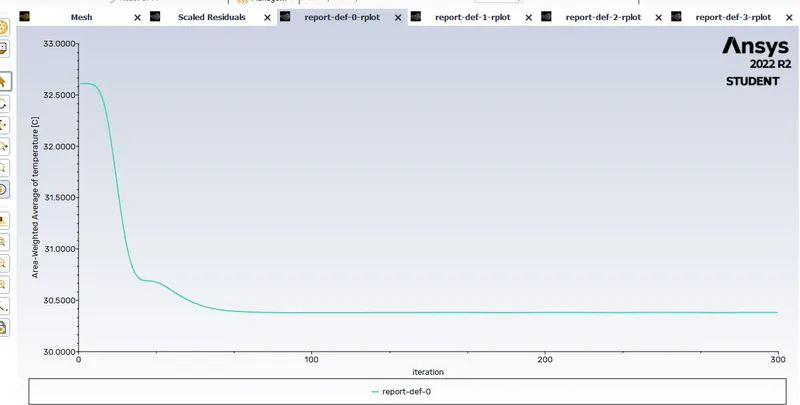
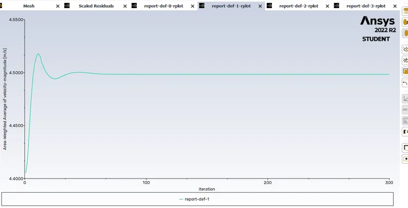
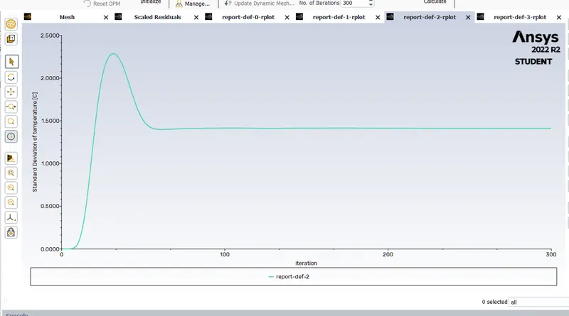
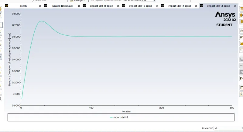
then in the solution part in reports the area weighted average of velocity and temperature at outlet, and standard deviation of temperature and velocity at outlet are created. and then the solution is initialisation hybrid method at t=0. after initialization calculations are run for 300 iterations. On the 159^th iteration the result was converged.

moment ratio 2 short T

moment ration 4 short T

K-epsilon short T

parameters	Inlet-x	Inlet-y	Area weighted average at outlet	Standard deviation
Temperature	36	19	30.4 C	2 C
Velocity	3	6	4.5m/s	.62 m/s

K-omega SST

parameters	Inlet-x	Inlet-y	Area weighted average at outlet	Standard deviation
Temperature	36	19	30.4 C	2.1 C
Velocity	3	6	4.5m/s	.65 m/s

Short T with standard mesh and with moment ratio 4

K-omega SST

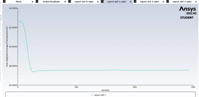
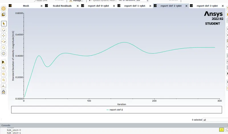
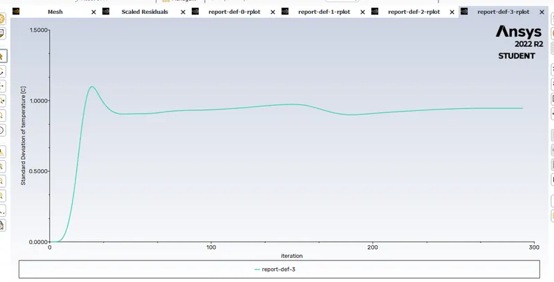
parameters	Inlet-x	Inlet-y	Area weighted average at outlet	Standard deviation
Temperature	36	19	27.5 C	.94 C
Velocity	3	12	6 m/s	.47 m/s

K-epsilon

.

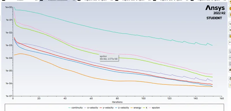
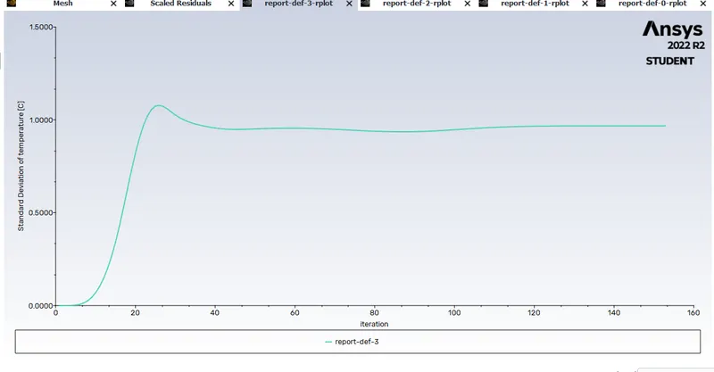
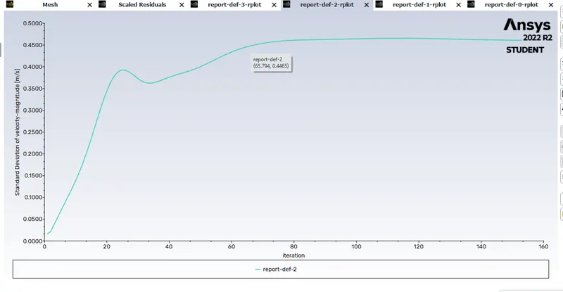
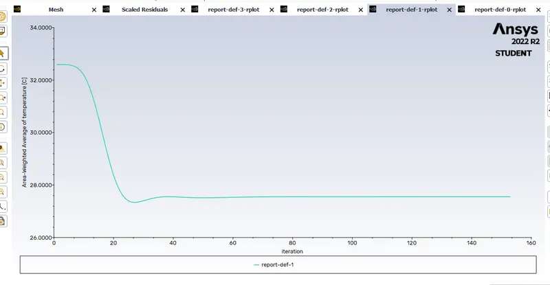
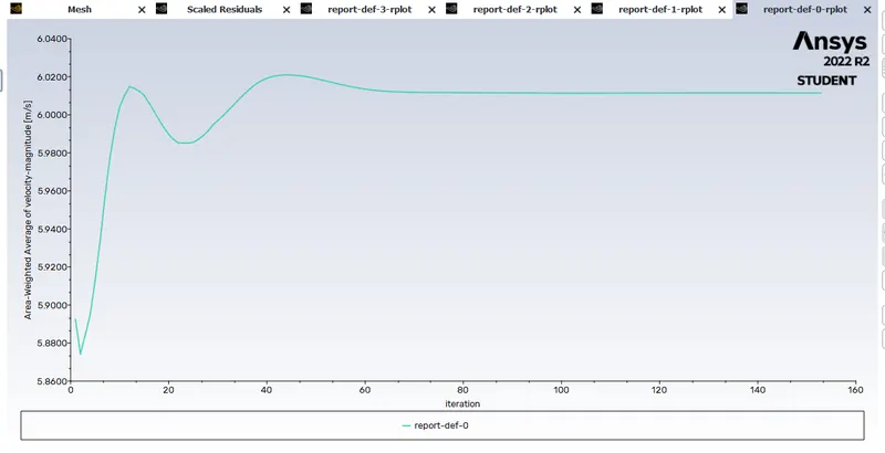
K-epsioln

parameters	Inlet-x	Inlet-y	Area weighted average at outlet	Standard deviation
Temperature	36	19	27.58 C	0.96 C
Velocity	3	12	6 m/s	0.46m/s

while solving the mixing in both K-Epsilon ad in k-omega SST, it is found that the k= epsilon has produced a converged value faster than K-omega SST model. The iteration required to reach convergence in K-epsilon is lesser compared to that of k-omega. In K-epsilon model the convergence occurs around 100th iteration an from there even though there is slight variation it is still ina steady manner is negligible. Also the result of both are almost identical and so K-epsilon is used for the further processing of the mixing in long T. by using K=epsilon we can save time and reduce machine run time cost.

Long T

parameters	Inlet-x	Inlet-y	Area weighted average at outlet	Standard deviation
Temperature	36	19	30.4 C	1.42C
Velocity	3	6	4.5 m/s	0.6m/s

Post processing :

After solving go to solutions in workbench and open CFD post to analyse the results along the T.

CFD post walls > render > set the transparency value for the walls and apply

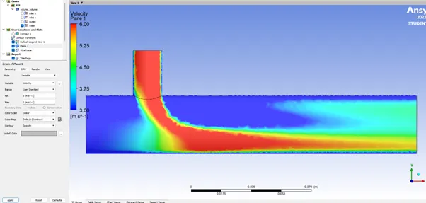
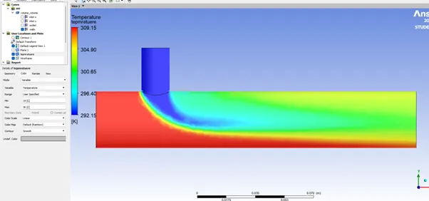
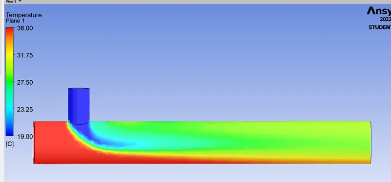
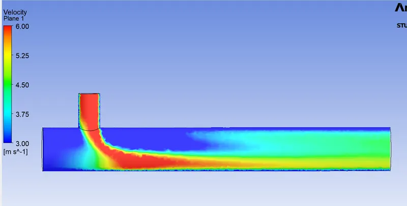
Then make a cut plane along the pipe in XY planes to analyse the temperature and velocity flow along the pipe.

In the colour set variable as Temperature and velocity and analyse the results.

moment ratio 2 short T

Moment ratio 4 short T K=omega SST

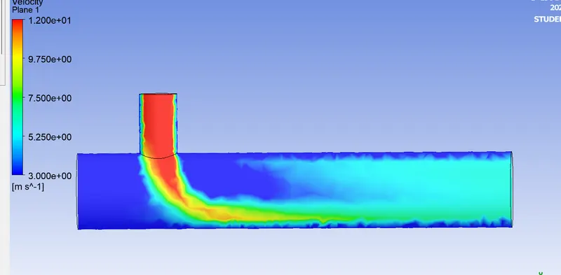
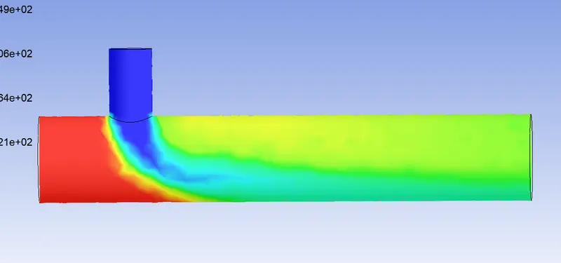
K-epsilon

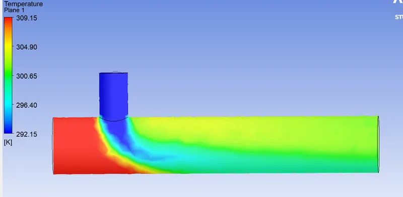
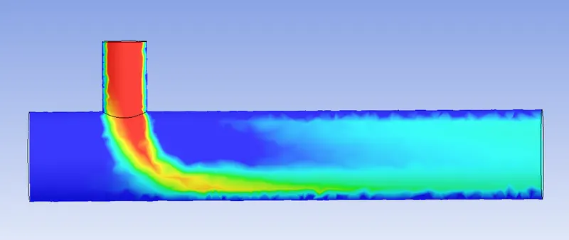
long T with moment ratio 2

Result:

T	Avg. temperature	cell count	no of iteration fro convergence
short		213356	100
long	30.4	140942	150

Analysis of mixing of air at different teperature in a T was conducted under bvarious moment ratio and using 2 viscous solution methods.

the solution was then plotted along the T to analyze the effect of mixing inside the T

Conclusion : it was found that when the mesh is refined the solution in both K=epsilon and K-omega SST is identical but K-epsiolon seems to rpovide a faster convergence than in the k+omega SST model. so for analyzing the mixing characteristics inside the T it is better to use K-eosilon thus allowing us to save time on computing and save computational expenses.