Studying Various cases of simulation in a Mixing Tee using ANSYS Fluent

Week 1 Report

• Aim: To Simulate the different cases of a Mixing Tee for two different Inlet Temperatures at two different Momentum Ratio for two different Lengths of the Mixing Tee and then to measure the Outlet Temperature of the working fluid, which in our case is air.
  
  
  
  
  
• Theoretical Introduction:
  
  Mixing Tees utilizes a specifically engineered internal geometry to efficiently mix two fluid streams into one combined stream. Mixing Tees are ideal for microbore or analytical gradient HPLC. These mixing tees are specifically designed for high-pressure applications.
  

  Mixing tees are widely used in the petrochemical industry, in which two fluid streams with different physical and/or chemical properties mix together. When there is a large temperature difference between the two streams, large metal temperature fluctuations can occur in the region where the two streams meet if proper design steps are not taken. The temperature fluctuations in the metal may lead to thermal fatigue of the pressure boundary piping. If through-wall cracking occurs, the fluid may leak, possibly causing a fire and damage. It is therefore imperative to make sure that the temperature fluctuations are such that the piping system can withstand them. Options can include improving the mixing of the two streams to reduce the temperature fluctuations through redesign of the piping system such that the momentum ratio of the two fluid streams is favourable to rapid mixing or to install devices that protect the pressure boundary piping, e.g., injection quills or thermal sleeves in the region where the temperature fluctuations are higher than a thermal fatigue threshold. This region includes the T-junction and a length of several to many main pipe diameters downstream from the T-junction.

  Empirical correlations in the literature may be used to estimate mixing effectiveness or the uniformity of the fluid concentrations over the pipe cross-section downstream from the T-junction, whereby the length of the pipe that needs protection can be determined. However, these correlations were developed based on experiments typically using air or water as working fluids and a chemical agent as the tracer to indicate the mixing uniformity. The temperature differences between the two fluid streams in these experiments were usually small. Therefore, these correlations should be used with caution when the actual fluid conditions are well outside of the range in which the correlations were developed.

  Computational fluid dynamics (CFD) modelling, such as well-resolved large eddy simulation (LES), can provide accurate predictions of the mixing behaviour, including velocity, concentration and temperature fields, in a mixing tee. The variations of the transient fluid temperature can therefore be used to identify a location in the main pipeline, after which the maximum temperature difference is less than a given value.

  
  
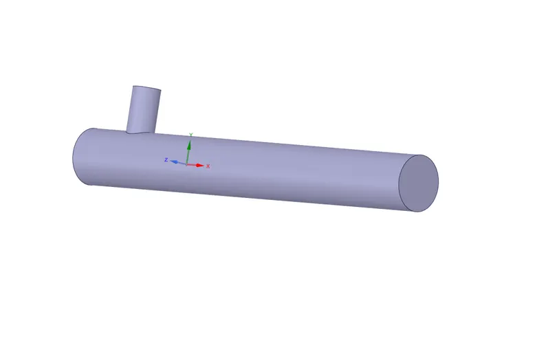
  Typical Example of a Long Mixing Tee
  
  
  Turbulence Models: Turbulence modelling is the construction and use of a mathematical model to predict the effects of turbulence. Turbulent flows are commonplace in most real-life scenarios, including the flow of blood through the cardiovascular system, the airflow over an aircraft wing, the re-entry of space vehicles, among others. In spite of decades of research, there is no analytical theory to predict the evolution of these turbulent flows. The equations governing turbulent flows can only be solved directly for simple cases of flow. For most real-life turbulent flows, CFD simulations use turbulent models to predict the evolution of turbulence. These turbulence models are simplified constitutive equations that predict the statistical evolution of turbulent flows
  
  A few of the examples for Turbulence models is given below:
  

  The Spalart–Allmaras model is a one-equation model that solves a modelled transport equation for the kinematic eddy turbulent viscosity. The Spalart–Allmaras model was designed specifically for aerospace applications involving wall-bounded flows and has been shown to give good results for boundary layers subjected to adverse pressure gradients. It is also gaining popularity in turbomachinery applications.

  • k–ε (k–epsilon)

  K-epsilon (k-ε) turbulence model is the most common model used in computational fluid dynamics (CFD) to simulate mean flow characteristics for turbulent flow conditions. It is a two-equation model which gives a general description of turbulence by means of two transport equations (PDEs). The original impetus for the K-epsilon model was to improve the mixing-length model, as well as to find an alternative to algebraically prescribing turbulent length scales in moderate to high complexity flows.

  • k–ω (k–omega)

  In computational fluid dynamics, the k–omega (k–ω) turbulence model is a common two-equation turbulence model that is used as a closure for the Reynolds-averaged Navier–Stokes equations (RANS equations). The model attempts to predict turbulence by two partial differential equations for two variables, k and ω, with the first variable being the turbulence kinetic energy (k) while the second (ω) is the specific rate of dissipation (of the turbulence kinetic energy k into internal thermal energy).

  • SST (Menter’s Shear Stress Transport)

  SST (Menter's shear stress transport) turbulence model is a widely used and robust two-equation eddy-viscosity turbulence model used in computational fluid dynamics. The model combines the k-omega turbulence model and K-epsilon turbulence model such that the k-omega is used in the inner region of the boundary layer and switches to the k-epsilon in the free shear flow.

  • Reynolds stress equation model

  The Reynolds stress equation model (RSM), also referred to as the second-moment closure model, is the most complete classical turbulence modelling approach. Popular eddy-viscosity based models like the k–ε (k–epsilon) model and the k–ω (k–omega) models have significant shortcomings in complex engineering flows. This arises due to the use of the eddy-viscosity hypothesis in their formulation. For instance, inflows with high degrees of anisotropy, significant streamline curvature, flow separation, zones of recirculating flow or flows influenced by rotational effects, the performance of such models are unsatisfactory. In such flows, Reynolds stress equation models offer much better accuracy.

  Eddy viscosity based closures cannot account for the return to isotropy of turbulence, observed in decaying turbulent flows. Eddy-viscosity based models cannot replicate the behaviour of turbulent flows in the Rapid Distortion limit, where the turbulent flow essentially behaves like an elastic medium.

  
  
  
  
  
  
• Procedure:
  
  1. The very first step would be to import the model in ANSYS Space Claim to edit the model according to the Geometry where the airflow is going to take place.
  To open this part in the workbench, we simply use the Geometry tab as shown below: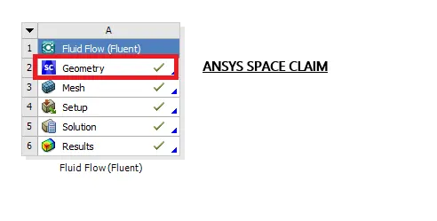
  
  
  
  After opening this, we have to extract the volume where the Air-flow is going to occur. To do this, we can use the Volume Extract option in the Prepare tab and use the Select edges option.
  
  This option will limit our Geometry and also help us mesh the required area under study much better. We must also deactivate the other Shell portion for Physics so that this region is not considered for the study.
  
  
  
  2. After preparing the model in Space Claim, the next step would be to mesh the model. In this tab as well, we must name the two Inlets and Outlet of the pipe.
  To name the Inlet and Outlet, we simply have to use the Ctrl+F option to select the Face that will act as the inlet and the Outlet for this simulation. We know where the Cold Air and the Hot Air Inlet are present and must name them accordingly. The naming of these faces will determine the Boundary conditions accordingly, although they can be changed if something wrong is detected by the ANSYS software.
  
  The naming of the Faces is shown below: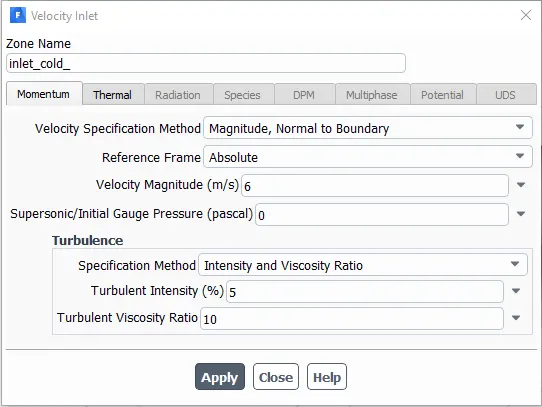
  
  
  Cold Air Inlet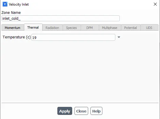
  
  
  
  Cold Air Temperature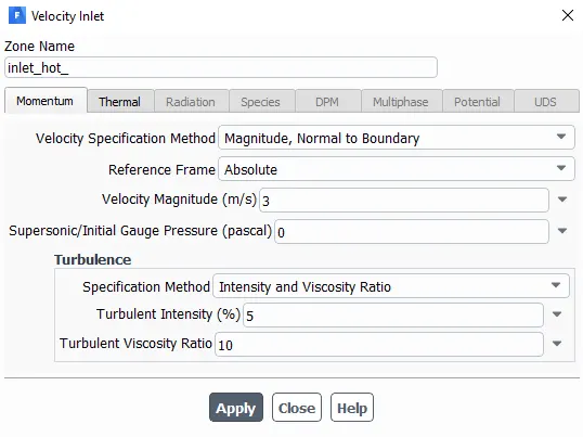
  
  
  
  
  Hot Air Inlet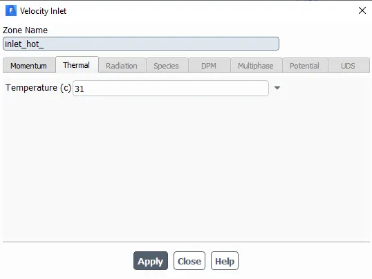
  
  
  
  
  Hot Air Temperature
  
  
  
  
  
  3. Another Important step is to request the Reports of the Area-weighted-Average and the Standard-Deviation of the Temperature as the variable on the Outlet.
  To request these reports, we use the Solutions tab inside the Setup part of the Fluent workbench.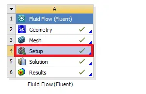
  
  
  
  In this module of the workbench, we can set up the problem as we desire. In our case, the only thing we wish to change is the Turbulence model and the Velocity of the Cold air inlet according to the Momentum Ratio that we wish to simulate the model with.
  
  Momentum Ratio can be defined as:
  
  Velocity at the Cold Air inlet / Velocity at the Hot Air Inlet
  
  We need to request the Reports from the Solutions tab in this module as shown: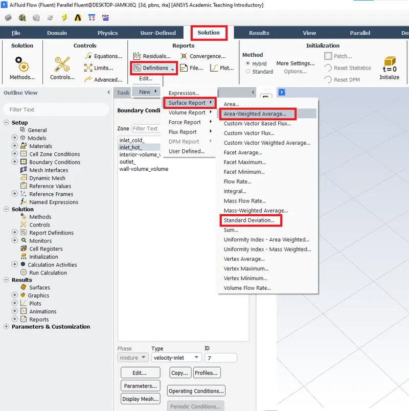
  
  
  We simply need to define the variable as Temperature and the boundary surface as the Outlet. The solver will then measure the Weighted Average Temperature at the Outlet and even the Standard Deviation at the outlet.
  
  
  The Reports can be checked as in the Edit tab for the same: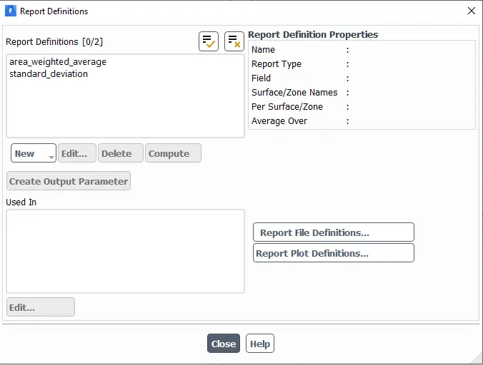
  
  
  As we can see that both the Area weighted Average and the Standard Deviation report has been requested successfully. We just need to make sure to click and check the Report Plot and Report File shown below: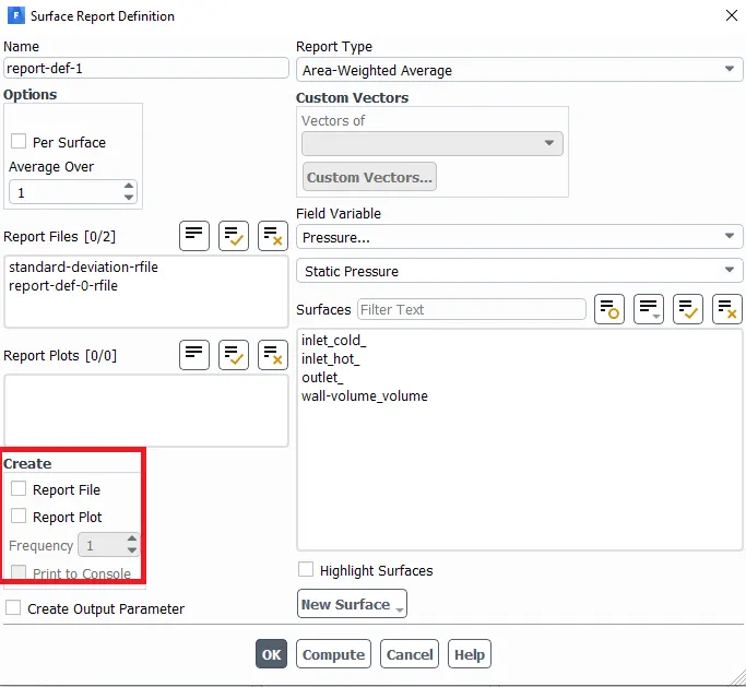
  
  
  
  
  
  
  
  
  4. After the Report Requests were made properly, the next step would be to initialize and then perform the appropriate calculations for the required number of time-steps.
  To Initialize, the following button must be used and then use the calculate button after setting the Number of Iterations we would want our simulation to run.
  
  
  
  
  
  
  5. The Iterations stop after the solution has converged. The Convergence criteria are as shown below: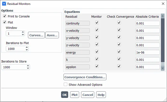
  
  
  
  The Absolute Criteria acts as a Tolerance level for the simulation.
  
  
  
  
  6. The cases for which we are supposed to perform the Simulation are as follows:
  
  a. Short Tee:
  
  a.1) M= 2
  
  a.1.1) Using the K-epsilon Turbulence Model.
  a.1.2) Using the K-Omega Turbulence Model.
  
  a.2) M= 4
  
  
  b. Long Tee:
  
  b.1) M= 2
  b.2) M= 4
  
  
  c.) Grid Independence Test on any one of the Cases.
  
  
  
  
  7. The simulation is performed according to Cases and setting up the case set up as demonstrated in all the procedure steps above.
  
  The next step is to plot the various planes and lines to plot the necessary charts.
  To plot the planes on the wireframe of the Selected volume, we must use the option of Location in the Results or the CFD post Tab in the workbench.
  In this module, we must use the tab of Location and then use the planes option as shown below: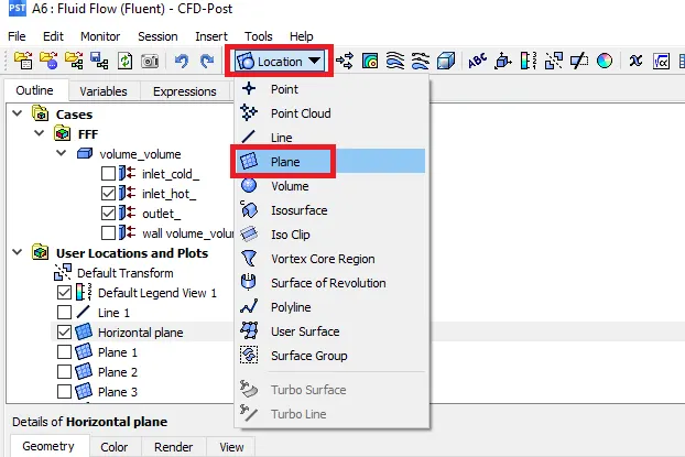
  
  
  
  Here, we must carefully select the location of the plane using the Global Axes and the length of the pipe etc.
  
  
  
  The result of this will be as follows: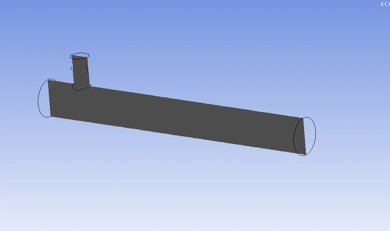
  
  
  
  
  Now, on this plane, we must colour the plane according to the variable that we need to measure. This variable can be Pressure, Temperature or even the Velocity of the simulation.
  
  Just like this, we must plot all the other planes across the Mixing Tee and even plot the line and then use the chart command to plot a certain variable measured across the line.
  
  
  All the Results for all the cases in the mixing Tee are explained below:
  
  
  
  
  
  
  
  
  
  
  

Results:

a. Short Tee:

a.1.1) K-epsilon turbulence Model for Momentum Ratio of 2.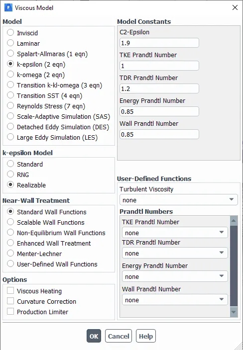



K-epsilon settings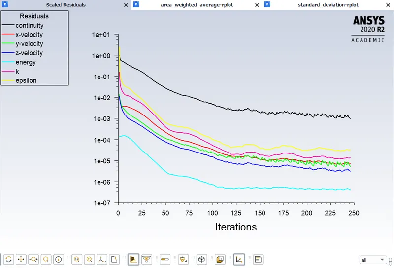



Convergence Plot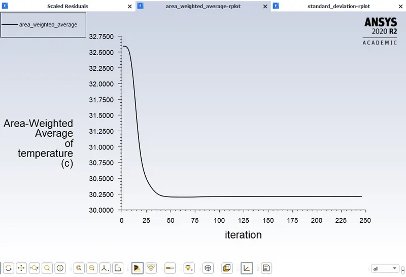



Area-weighted-Average of Temperature.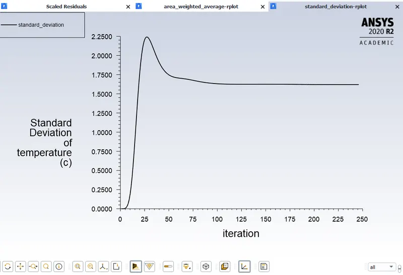



Standard Deviation for the simulation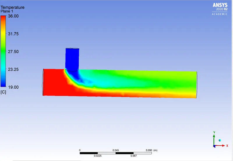



Temperature Distribution

The Temperature Distribution plot is shown in the plane above. We can see that as the air moves along the length of the mixing tee, the convection of the air leads to the mixing of air and thereby a mixture of the two temperatures at the outlet. From the Area-weighted-average, we can see that the Outlet temperature is approximately 30.25-degrees celsius.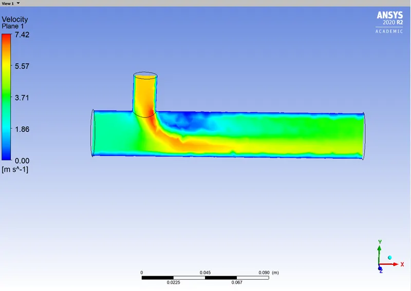



Velocity Distribution

The velocity plot is shown above.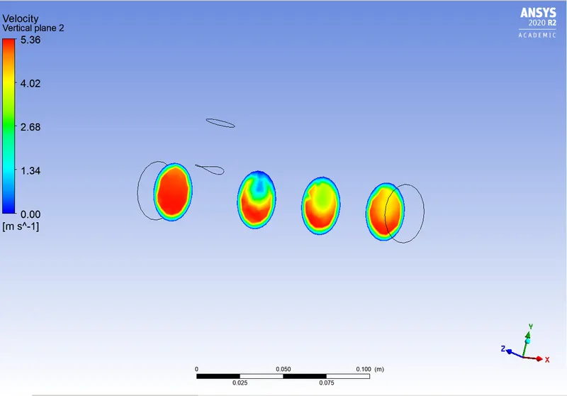



Velocity Distribution across the Mixing Tee.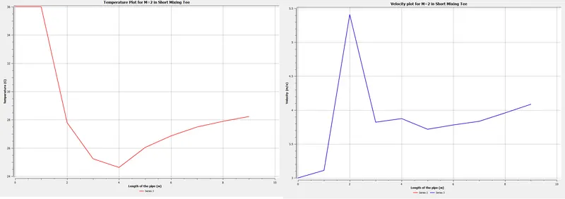




Temperature and Velocity plots

The Temperature decreases as soon as the mixing starts and then decreases till a certain point and then starts to increase gradually till the outlet.
The Velocity plot is again the same, the magnitude increases as soon as the two temperatures of air mix and then it starts to settle and become much less as the convection occurs in the model.



a.1.2) K-omega turbulence Model for Momentum Ratio of 2.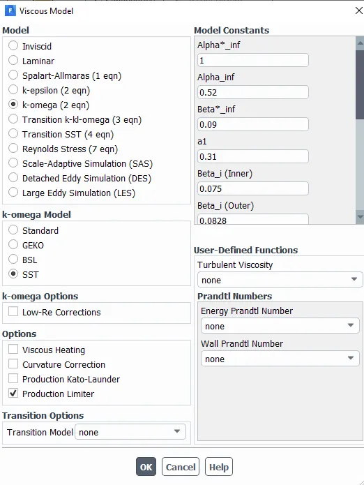



K-omega setting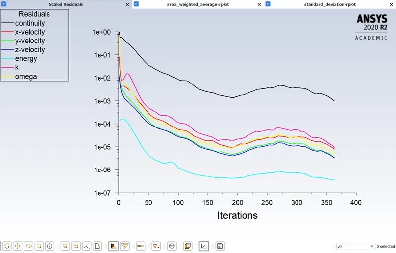



Convergence plot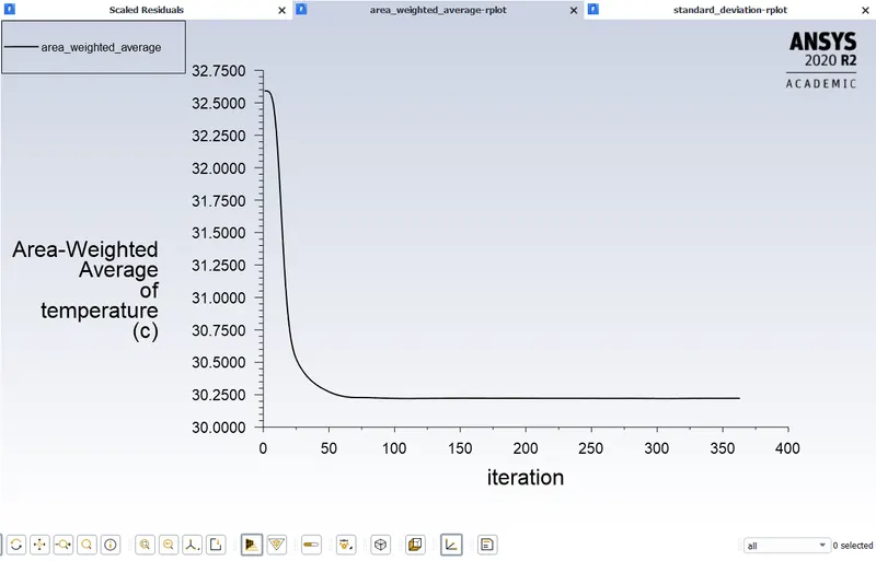




Area-weighted-average of temperature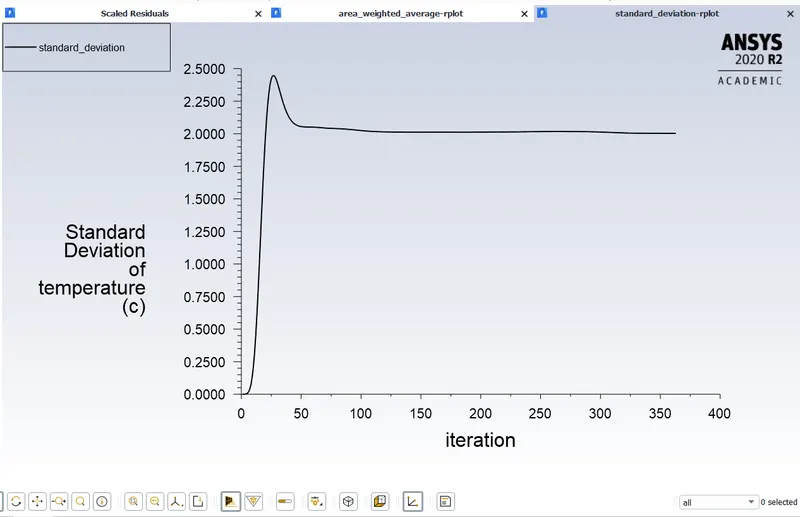



Standard Deviation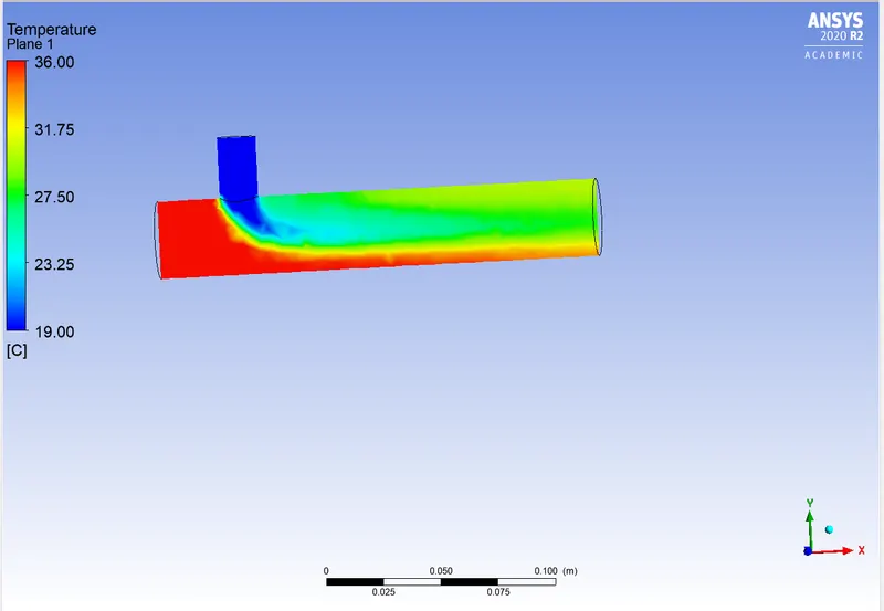



Temperature Distribution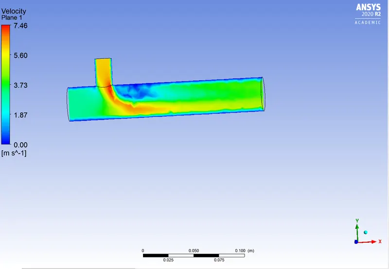



Velocity Distribution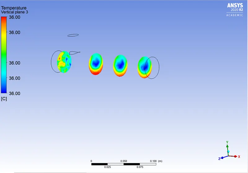



Temperature distribution across the Mixing Tee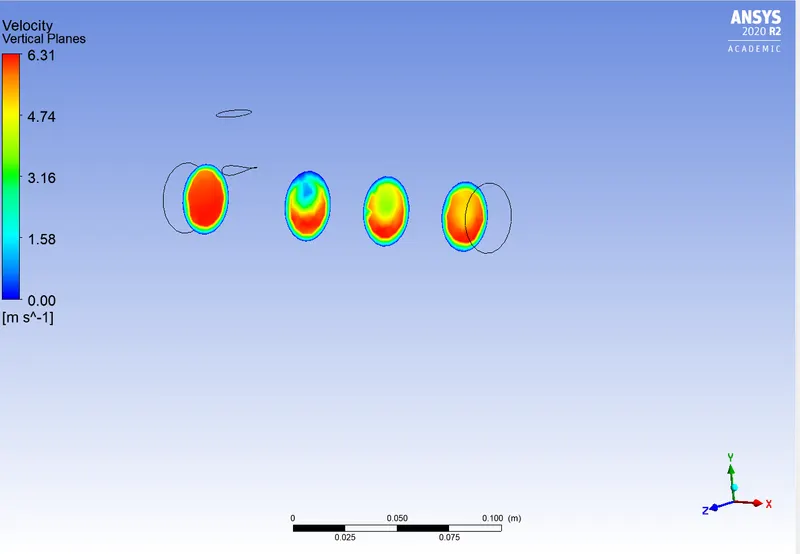



Velocity distribution across the Mixing Tee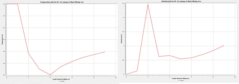




Temperature and Velocity plots


The Difference between the K-epsilon and the k-omega turbulence model is that the K-epsilon model predicts well far from the boundaries (wall) and the k- omega model predicts well near the wall.

The k stands for Kinetic Energy and the epsilon is for the Turbulent Dissipation. Turbulent dissipation is the rate at which velocity fluctuations dissipate. In the standard k-e model, the eddy viscosity is determined from a single turbulence length scale, so the calculated turbulent diffusion is that which occurs only at the specified scale, whereas in reality, all scales of motion will contribute to the turbulent diffusion. The k-e model uses the gradient diffusion hypothesis to relate the Reynolds stresses to the mean velocity gradients and the turbulent viscosity. Performs poorly for complex flows involving severe pressure gradient, separation, strong streamline curvature.

A two-transport-equation model solving for kinetic energy k and turbulent frequency ω. This is the default k–ω model. This model allows for a more accurate near-wall treatment with an automatic switch from a wall function to a low-Reynolds number formulation based on grid spacing. Demonstrates superior performance for wall-bounded and low Reynolds number flows. Shows potential for predicting transition. Options account for transitional, free shear, and compressible flows. The k-e model uses the gradient diffusion hypothesis to relate the Reynolds stresses to the mean velocity gradients and the turbulent viscosity.

The Number of Iterations for the solution to converge is also less in K-`epsi`model, for the first case where we took M=2 in a short mixing Tee, the Number of Iterations for the solver to converge the solution is 250 whereas in the case of k`omega` the number of iterations required for the solver to converge the solution, is 363 precisely.


a.2) Short Mixing Tee for Momentum ratio = 4.

As the Momentum ratio is 4 in this case, the Speed of the Cold air at the inlet increases from 6 in the previous case to 12 in this. We then perform the simulation and then understand the difference between these two cases.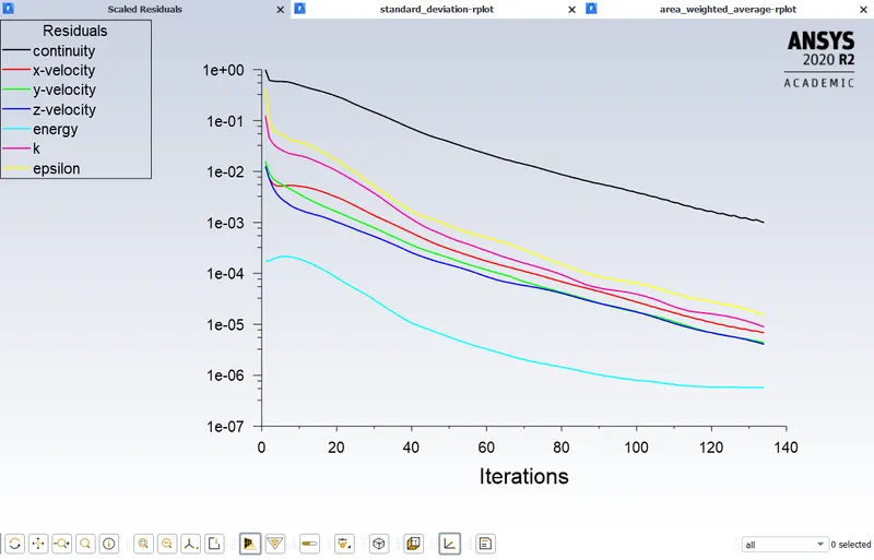



Convergence Plot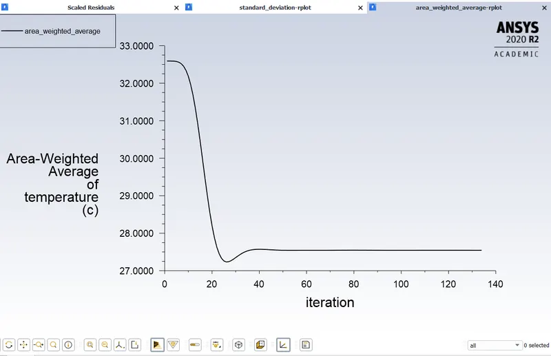



Area-weighted-average of Temperature

The Temperature at the outlet will be lesser than the one we got in the previous case. This is because the velocity of the cold air at the inlet is twice in this case when we compare it with the previous case. So, for the same length of the pipe, more amount of air is flowing through the inlet. The Mass flow rate has a formula of `rho * A * v`where, v is the velocity of the fluid flowing. Since the velocity has increased, more mass will be flowing through the inlet therefore the temperature measured at the outlet will be even less.
This can be confirmed with our simulation results as well.

For M=4, the outlet temperature is approximately equal 27.5-degree celsius
For M=2, the outlet temperature is approximately equal to 30.25-degree celsius.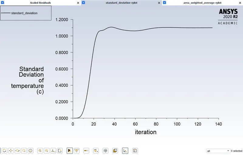



Standard-Deviation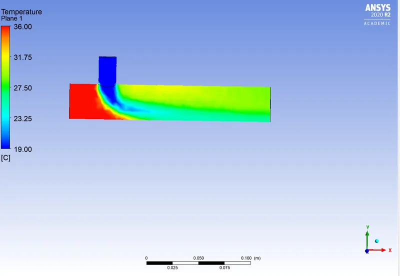



Temperature Distribution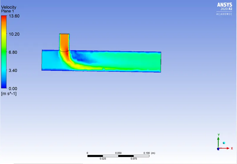



Velocity Distribution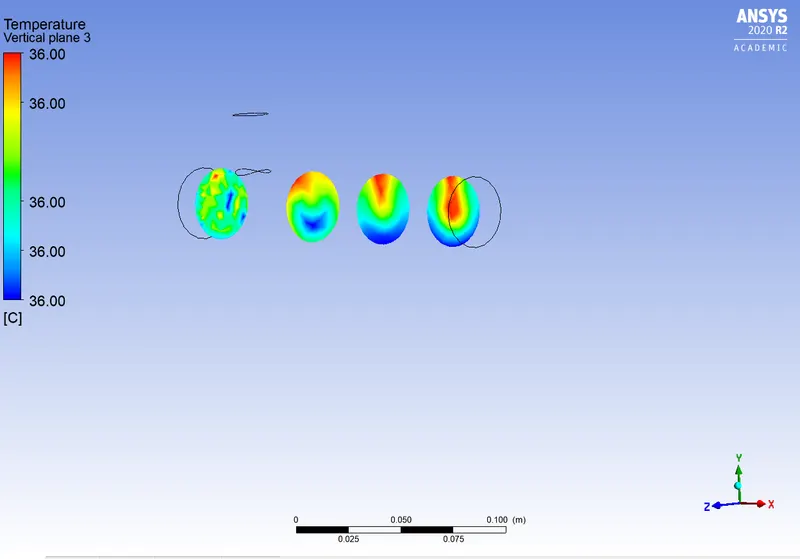



Temperature Distribution across the Mixing Tee

As the simulation progresses and the two airflows at two different temperatures are mixing and convection is occurring, we can see that the Temperature is getting more and more uniform.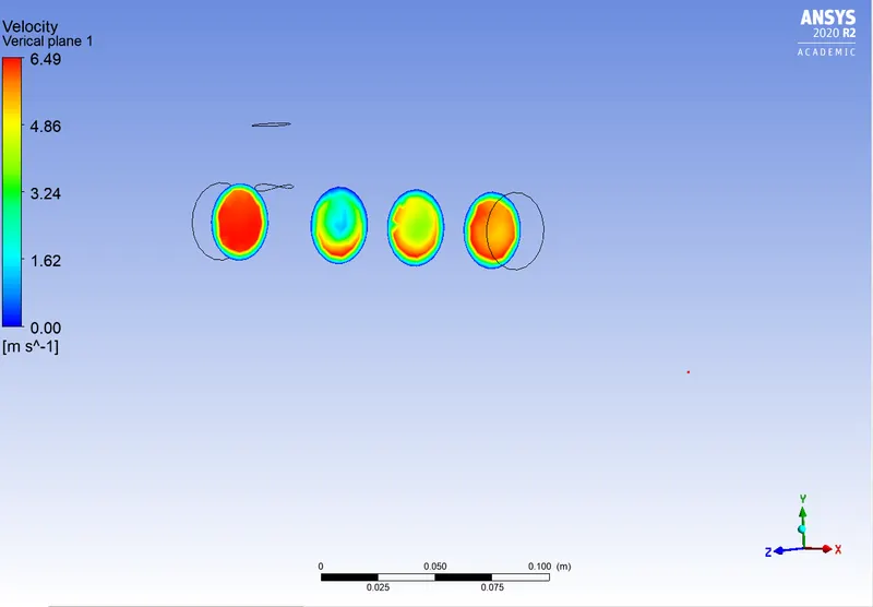



Velocity Distribution across the Mixing Tee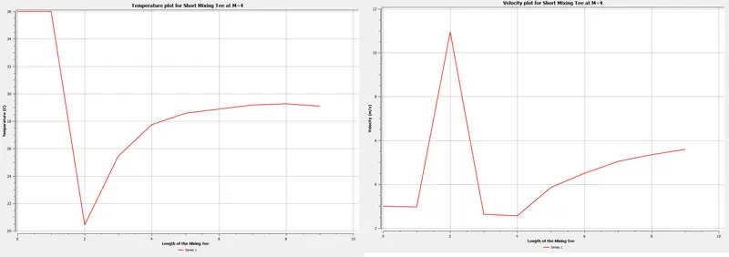



Temperature and Velocity Plots

We can see that at the exact point where the velocity is increasing along the line for which we are extracting the plots as the air is flowing at 12m/s for the cold temperature and since the temperature is lesser than the hot air that is flowing through the other inlet, there is a temperature drop that is being observed in the Temperature plot.




b.1) Momentum ratio for the Long Tee

The results are as follows: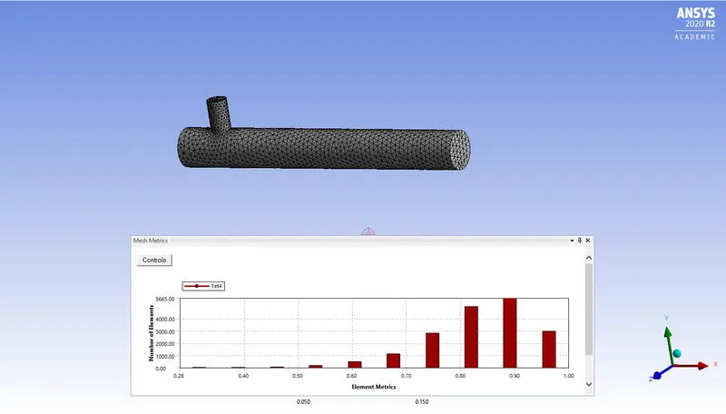



Quality check for the mesh




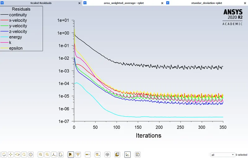
Convergence Plot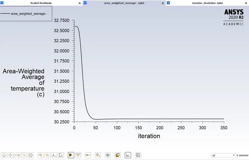



Area-weighted-Average of Temperature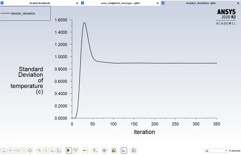




Standard Deviation of Temperature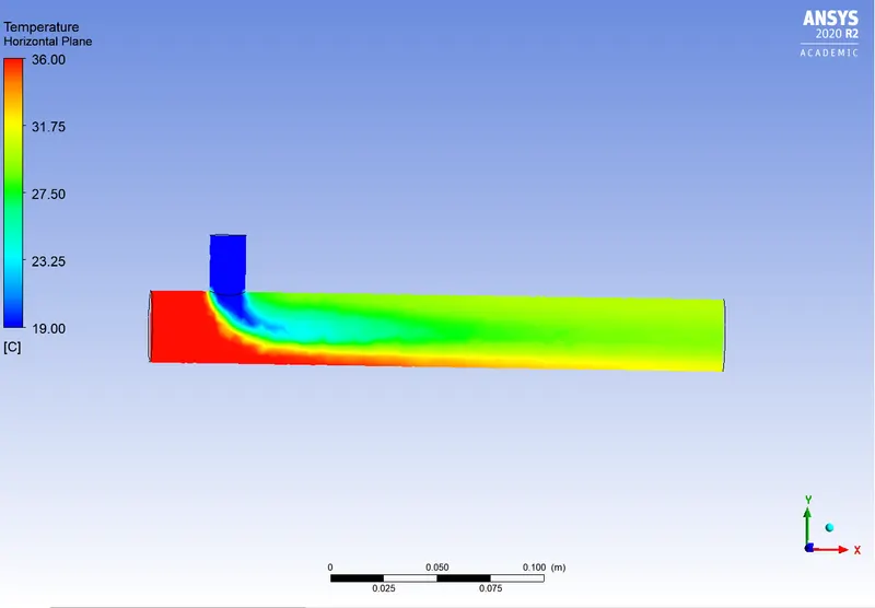



Temperature Distribution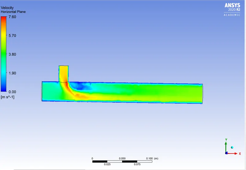



Velocity Distribution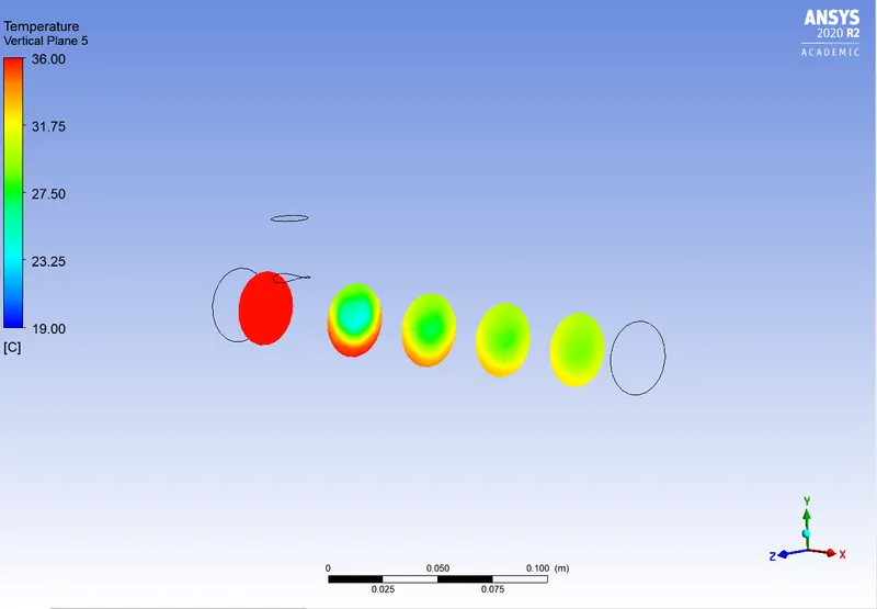




Temperature Distribution across the Mixing Tee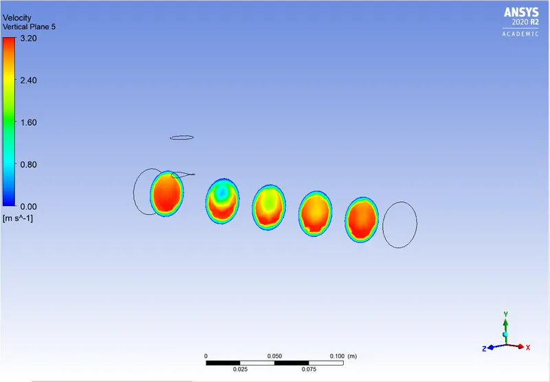



Velocity Distribution across the Mixing Tee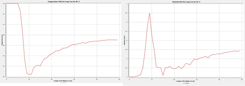



Temperature and Velocity Plots



b.2) M=4 in a Long Mixing Tee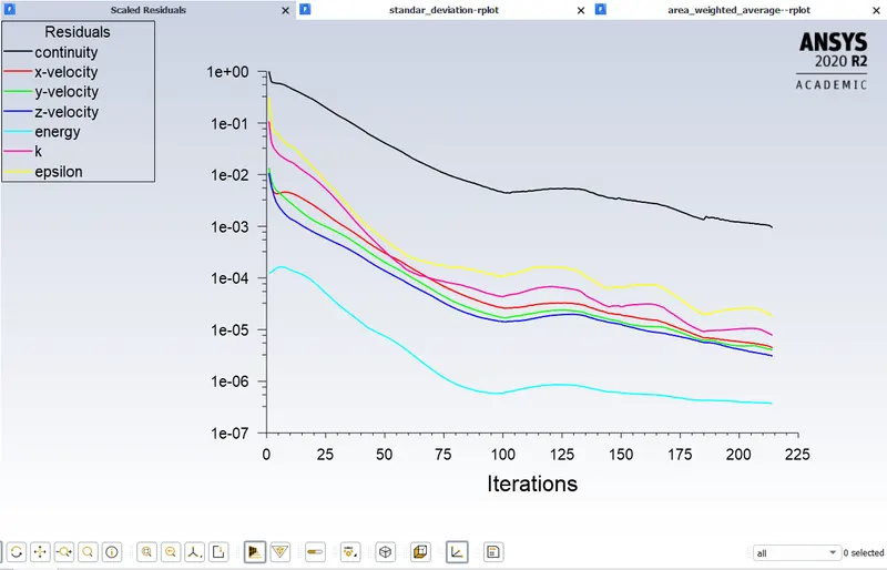



Convergence Plot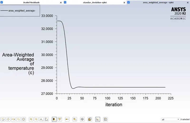




Area weighted Residual of Temperature

The Temperature at the outlet will be lesser than the one we got in the previous case. This is because the velocity of the cold air at the inlet is twice in this case when we compare it with the previous case. So, for the same length of the pipe, more amount of air is flowing through the inlet. The Mass flow rate has a formula of `rho * A * v`where, v is the velocity of the fluid flowing. Since the velocity has increased, more mass will be flowing through the inlet therefore the temperature measured at the outlet will be even less.
This can be confirmed with our simulation results as well.

For M=4, the outlet temperature is approximately equal 27.5-degree celsius
For M=2, the outlet temperature is approximately equal to 30.25-degree celsius.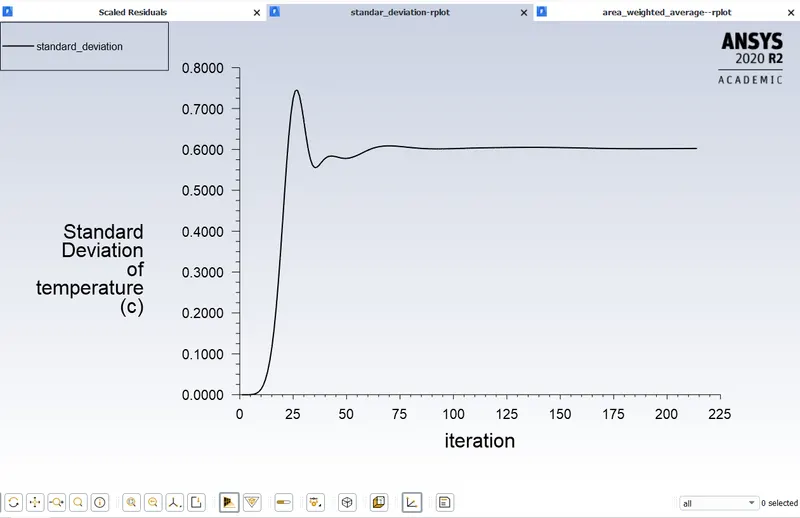



Standard Deviation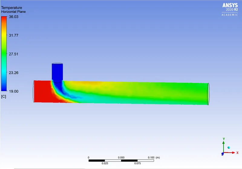



Temperature Distribution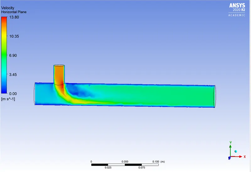



Local Velocity Distribution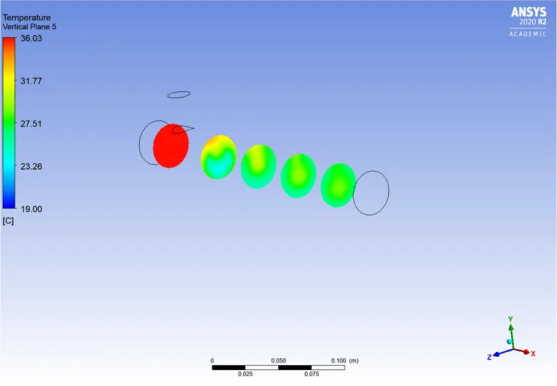



Temperature distribution across the Mixing Tee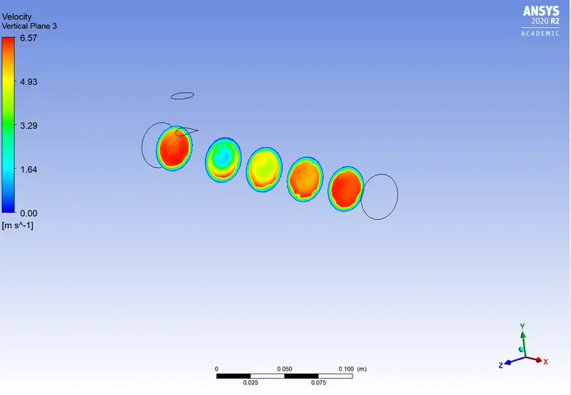



Velocity distribution across the Mixing Tee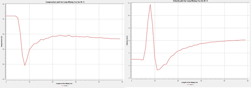



Temperature and the Velocity plots




c.) Grid Independence Test

The Grid Independence Test is done so as to check the dependency of the mesh on the Final Solution. The Accuracy will indeed change with the change of the mesh size, but the change in the accuracy should not be by a big margin.

We have taken three cases with a mesh size of 0.005, 0.01 and 0.5. The mixing Tee specifications are such that it is the long Mixing Tee with a Momentum Ratio of 4 and have deployed the K-epsilon Turbulence Model for the simulation. We then compare the results that we get in these cases.

All the plots shown are in the ascending order of the mesh lengths that we have used, i.e. 0.005, 0.01, 0.5.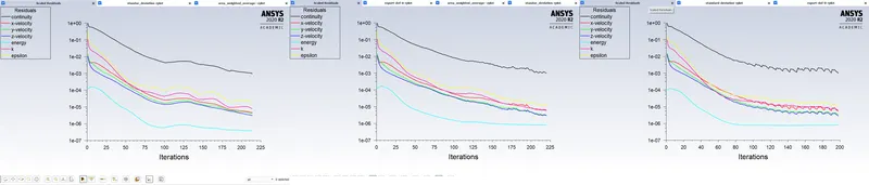



Plot for Scaled Residual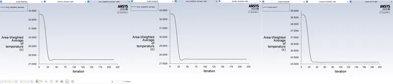



Plot for Area Weighted Average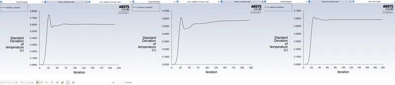



Plot for Standard Deviation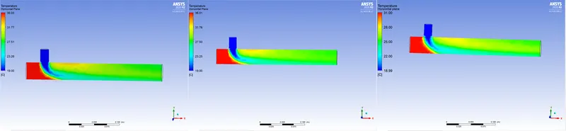



Temperature Distribution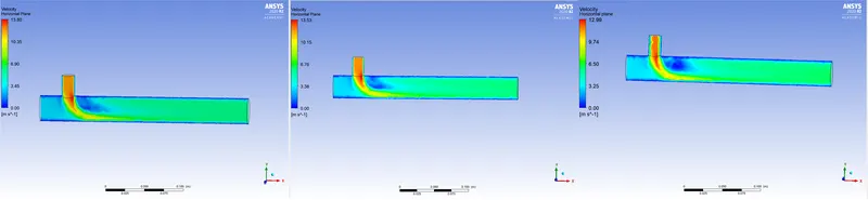



Velocity Distribution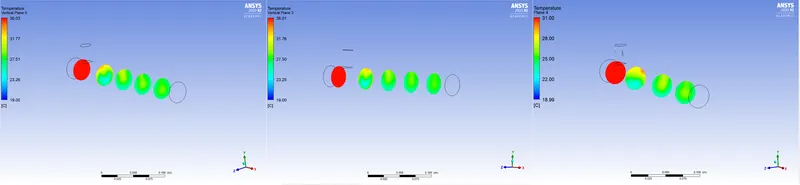



Temperature Distribution across the Long Mixing Tee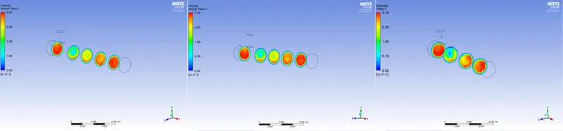



Velocity Distribution across the Long Mixing Tee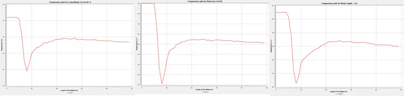



Temperature plot for all three cases.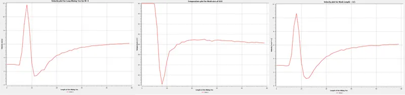



Velocity plot for all three cases.


As we can see that in all three cases, the change is very minute and that the Physics of the problem is also not changing. Yes, in the case of Mesh length equal to 0.5, the accuracy will have decreased due to the lesser number of elements in the geometry, but the solution is not really changing by a huge margin or completely in the opposite direction.

The table for the Number of Mesh Elements and Average Outlet temperature is given below:

	Momentum Ratio	Cell Count	Average Outlet Temperature(C)
Short Mixing Tee	2	12760	30.2
	4	12760	27.5
Long Mixing Tee	2	18173	30.2
	4	18173	27.5

From the table, we can draw conclusions between the length of the Mixing pipe and the Momentum Ratio that we are using. We can see that for the same momentum ratio, there is no change in the output temperature with an increase in the length of the Mixing Tee. Although the Standard Deviation is much lesser in the Longer Mixing Tee. This is because the Air has a much more length for it to undergo convection and mix much well before coming out of the outlet when compared to the shorter Mixing Tee. We can safely say that the length of the Mixing tee has no effect on the Output Temperature.


When we compare the Momentum Ratio is compared for the same length of the Mixing Tee, the increase in the momentum ratio results in a decrease in the Outlet Temperature because as the momentum ratio increases, the velocity of the Cold Air increases and due to this, the Mass flow rate increases thereby decreasing the Outlet Temperature of the air flowing out of the Mixing Tee. We can conclude that as the Momentum ratio increases, the Outlet velocity will increase.

• Validation:
  
  The Validation is done for a Short Tee with a Momentum ratio of 2.
  
  
  We know the formula:
  
  
  
  
  where,
  
  `m_(hot)` = Mass flow Rate of the Hot Air.
  
  `m_(cold)` = Mass flow of the Cold Air.
  
  `T_(cold)` = Temperature of the Cold Air.
  
  `T_(hot)` = Temperature of the Hot Air.
  
  `T_(mixture)` = Temperature of the Mixed Air.
  
  so,
  
  `m_(hot)` = `rho * A * v` = 1.225 * 0.0009 * 3 = 0.0033075 kg/s
  
  `m_(cold)` = `rho * A * v` = 1.225 * 0.0002 * 6 = 0.00147 kg/s
  
  Also, `T_(cold)`= `19^o`
  
  `T_(hot)` = `36^o`
  
  Applying the above-mentioned formula, we get the `T_(mixture)`= `30.77^o`
  
  And from the Simulation, we get the Temperature of the air mixture as `30.2^o`
  
  The Error = ((30.7-30.25)/30.7 ) *100 = 1.7% which is well below the maximum error that we can in a simulation.
  
  
  
  
  
  
• Conclusions: In conclusion, I would like to state that this challenge helped me gain a better understanding of the GUI of ANSYS Fluent and helped me understand how to set up a basic problem in it. I also understood the two turbulence modelling methods and how the length of the Mixing Tee and the Momentum Ratio of the Mixing Tee affects the Output Temperature.