Week 1- Mixing Tee

AIM -

A steady-state simulation is to be carried out in a mixing tee, for two cases - short tee & long tee, to compare the mixing effectiveness when the hot inlet temperature is 36°C & the cold inlet is at 19°C.

Case 1 -
Short mixing tee model with a hot inlet velocity of 3m/s.
Momentum ratio of 2, 4.
Case 2 -
Long mixing tee model with a hot inlet velocity of 3m/s.
Momentum ratio of 2, 4.

Momentum ratio = velocity at cold inlet/velocity at hot inlet

THEORY -

Mixing Tees are a simple and inexpensive way to provide chemical diffusion to a system. It employs a specially designed internal geometry to efficiently combine two fluid streams into a single combined stream.
Low viscosity mixing, such as wastewater treatment, the blending of some oils (injection of additives), and petrochemical products are examples of pipeline mixing with tees applications. Other uses include fuel gas blending and mixing of feed streams for catalytic reactors.


INTRODUCTION -

We are supposed to do steady-state simulation on the fluid domain, and not on the solid geometry. Here, we are mixing two fluids, that is, hot fluid and cold fluid, to find the mixing effectiveness, temperature of the mixed fluid, and temperature distribution & using line & contour plots. Upon completion of the simulation, we will compare the results from both cases and bring out the necessary conclusions regarding the mixing effectiveness, temperature distribution, etc. based on the length of the pipe and momentum ratios.


SOLVING & MODELLING APPROACH -

The flow of the entire process:

• Problem definition
• Pre-processing
• Solver or Processor
• Post Processing

In the problem statement, it is asked to perform the simulation on two models. We will consider these as two different cases. In each case, we need to simulate two momentum ratios - 2 & 4.
The hot inlet temperature is given as 36°C and the cold inlet temperature is given as 19°C.

Given that, Momentum Ratio = Velocity at the cold inlet / Velocity at the hot inlet
Here, in both cases, hot inlet velocity is given as 3 m/s.

For Momentum Ratio 2:

Cold inlet velocity will be 6 m/s

For Momentum Ratio 4:

Cold inlet velocity will be 12 m/s

Case 1 -
Short mixing tee with a hot inlet velocity of 3m/s.
Momentum ratio of 2, 4.
Case 2 -
Long mixing tee with a hot inlet velocity of 3m/s.
Momentum ratio of 2, 4.


Case 1 - Short Tee Model -

For Momentum Ratio = 2 -

Open the Ansys Workbench, and double click the "Fluid Flow (Fluent)". Rename the system as "Short Tee - MR 2".

PRE-PROCESSING -

Open the Spaceclaim by right click over the "Geometry File" option.

In Spaceclaim, we will extract the fluid volume.
Import the "Short Tee" model into the Spaceclaim.
Prepare > Volume Extraction > select 'Edges' option > select the three edges (two inlets & one outlet) > click the 'tick' symbol

Thus, a new volume is created.
Now we only need the fluid volume from this geometry and all the external surfaces need to be eliminated. Hence, we will use the "Suppress for Physics" command over the external solid surface. This command will not consider the outer surface of the model for further simulation.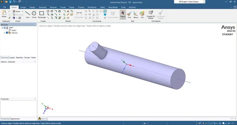




Further, we will mesh this model. For the same, close the Spaceclaim and in Ansys Workbench, click the "Mesh File".

Using a 3 mm element size we generated a volume mesh over the model.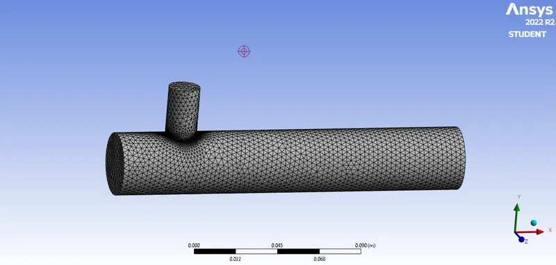

The finer the mesh, the more computational time it will take to give more accurate results.

Now, let's have a cut-section view of the model to view the volume mesh generation. Click the 'Sectional Plane' option and draw a simple line according to the desired cut.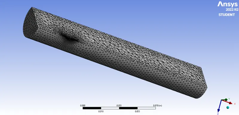



We need to define the proper boundaries of the model as inlets, outlets, and the wall as shown in the snapshot.

Select a particular face, right-click, click 'Apply selected geometry', write the exact name of that particular face which is to be assigned, and click OK.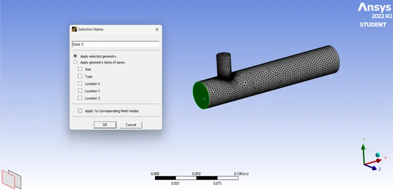



Now, Open the Ansys Workbench and click the "Setup File".

PROCESSING / SOLVER -

In the model, the blue rays indicate inlets and the red rays indicate outlets.

Under Domain toolbar set -
Solver Type: Pressure-based
Solver Velocity-Formation: Absolute
Solver Time: Steady

In the Display tool, we can see all the surfaces assigned to the model.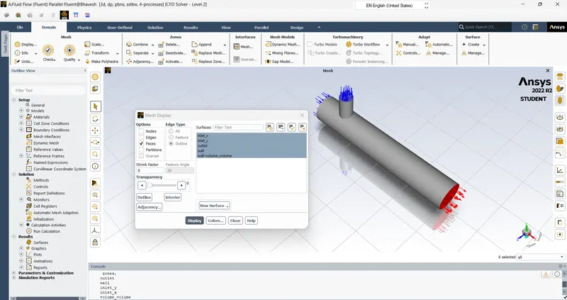



In the Units tool, we can change the units.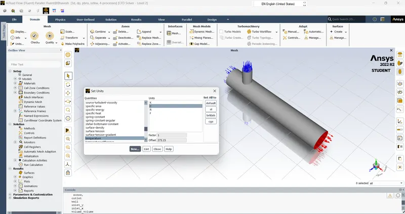



Under the Physics toolbar, enable the energy equation. In Viscous Model, select the k-omega model and the SST k-omega model. Click OK.

Note - The k-omega SST model is a combination of k-omega and k-epsilon. For near-wall and above-wall this model works better for simulation.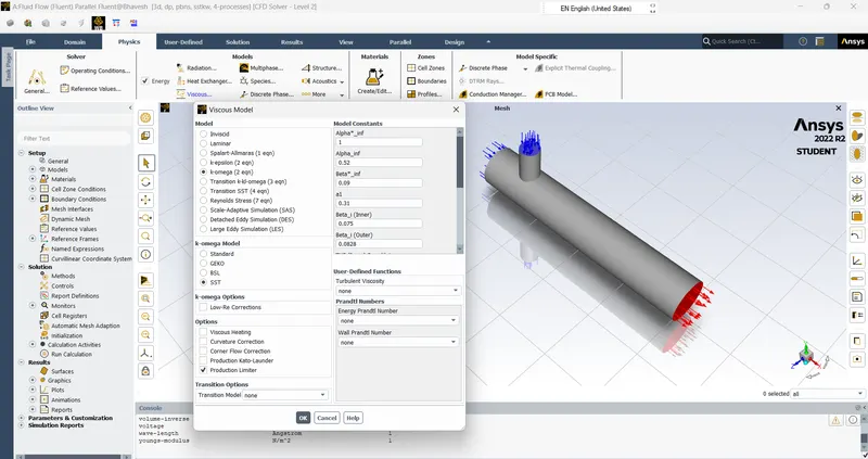



Under the Materials tool, the default material for fluid and solids are air and aluminum respectively. One can add other materials using 'Fluent Database' and 'User-defined Database' enables a user to add a new material with desired properties.

Under the Zones tool,

1. in Cell Zones, set Type - Fluid and edit Material name to 'Air'. Click apply.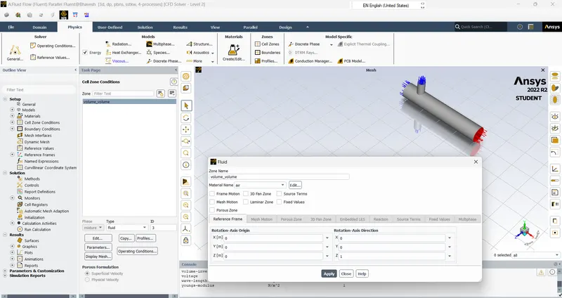



2. in Boundaries,

For inlet X:
Type = Velocity-inlet; under Momentum, Velocity Magnitude = 3 m/s and under Thermal, Temperature = 36°C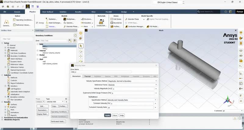



For inlet Y:
Type = Velocity-inlet, under Momentum, Velocity Magnitude = 6 m/s and under Thermal, Temperature = 19°C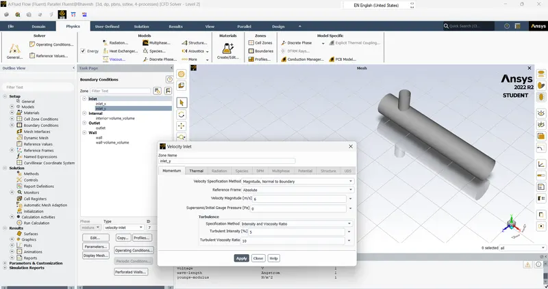



For Outlet:
Type = Pressure-outlet, Operating Conditions = 101325 Pa

Under the Solutions Toolbar, click the 'Initialize' button choosing the 'Hybrid' method.

Here, we are interested in contour plots and the average temperature at the outlet.

To generate the report -

Solution Toolbar > Reports > Definitions > New > Surface Report > Area-Weighted Average

Under Surface Report Definition, put -
Name: temperature
Field Variable: Temperature
Surfaces: Outlet
Enable 'Print to Console' & click OK.

Similarly, for the standard deviation of the temperature report, the same procedure needs to be followed.

In Outline View, one can see the temperature report and standard deviation report updated under 'Report Definitions'.

Now, we need to plot the contours or graphs of velocity and temperature at the initial conditions and we will plot it under the Results Toolbar.

Results > Graphics > Contour > Contour Name = Velocity > Contour Type = Velocity > select all the surfaces > click Save/Display

Repeat this for temperature too.

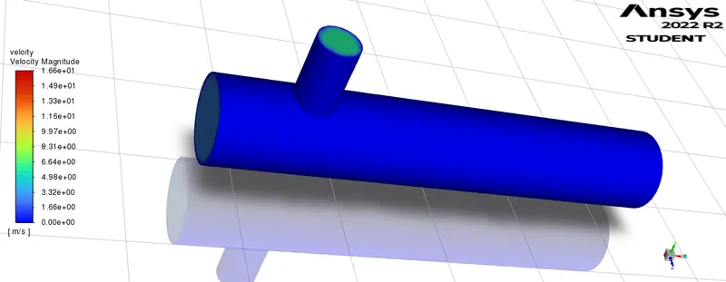
To see the cut sectional view, we need to create a plane.

Results > Surface > Create > Plane > Method = XY Plane

A plane will be created at the center by default and can be seen among the other surfaces enlisted.

Under the velocity contour, select the newly created plane and click Save/Display. This will show the initial values of velocity before starting the simulation, that is, before mixing the fluids.

Similarly, temperature contour can also be made.


Now, we will run the simulation for 150 iterations with the hybrid method. Here, it got converged at 111 iterations.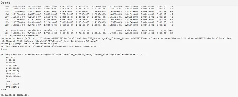

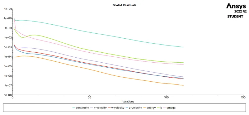
In case, if it does not converge under a given number of iterations, one may run the simulation for more iterations.

Now, we need to compute the values of temperature and standard deviation of temperature under the 'Reports Definitions'.

These are the values at the outlet,
Temperature = 30.344911° C
Standard Deviation = 1.8137723° C

For better mixing standard deviation should be low.

Now, we will find the minimum, maximum, and average values of velocity and temperature at the outlet.

Results Toolbar > Reports > Surface Integrals > Report Type = Facet Average > Field Variable = Velocity > Surfaces = Outlet > Compute

Compute for minimum and maximum values of velocity at the outlet in the same manner.

Similarly, find these values of temperature at the outlet.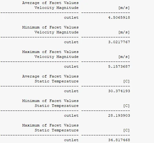



Velocity:

Average = 4.5065918 m/s
Minimum = 3.0217767 m/s
Maximum = 5.1573687 m/s

Temperature:

Average = 30.37419°C
Minimum = 28.193903°C
Maximum = 34.817468°C

Sr. No.	Parameter	Average	Minimum	Maximum
1.	Temperature (°C)	30.37419	28.193903	34.817468
2.	Velocity (m/sec)	4.5065918	3.0217767	5.1573687

To find the area of a particular surface, we may use the 'Projected Areas' tool under Results Toolbar.

Now, we will generate a report for our simulation.

Under Outline View, in 'Simulation Reports', click Report Outline and click Generate.

It will take some time as this report contains every detail right from system Information to the velocity & temperature contours.

One may export this report and save it as a PDF.

Now, we are supposed to carry out the post-processing to find the results.

POST-PROCESSING -

In Ansys Workbench, click the "Results File" and CFD-Postprocessor will open.

Note - One cannot open the 'Solution File' and the 'Result File' at a time.

Change the model from Wireframe mode to Volume mode. Here, one can color the external surfaces of the model with variables like temperature, pressure, etc.

Under Outline, double-click a particular surface, change the mode to Variable, variable to temperature and click apply.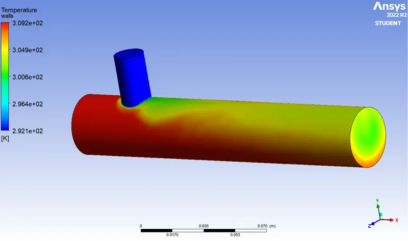



Let's create an XY plane using the 'Plane' command in the Location toolbar. By default, this plane will be created at the center of the model in the selected plane. We will color this plane using 'Temperature' as the variable.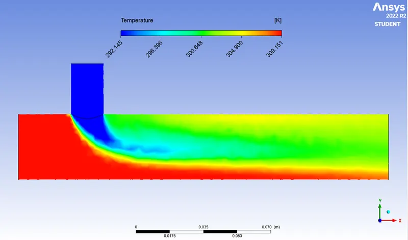



Similarly, we will create a 'Velocity' variable on this plane.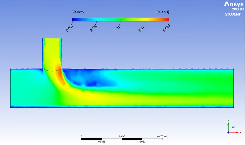



Now, we are supposed to plot graphs of velocity and temperature against the length of the flow (length of the pipe).

To plot a graph, first, we need to create a line.

Location > Line > give a specific name > OK Cut > Apply

A line will be created along the plane through the center. (Here, we will plot all the graphs on this line, such that the variations in values of temperature and velocity are with respect to this line.)

Now, to create a plot, click 'Chart', name it "Temp Plot", and click OK. Later, change the title, Data Series - Location as Line, X-axis as variable 'X-axis' and Y-axis as variable as 'Temperature'. Click apply.

A 'Temperature Vs Length of the flow' graph will be plotted.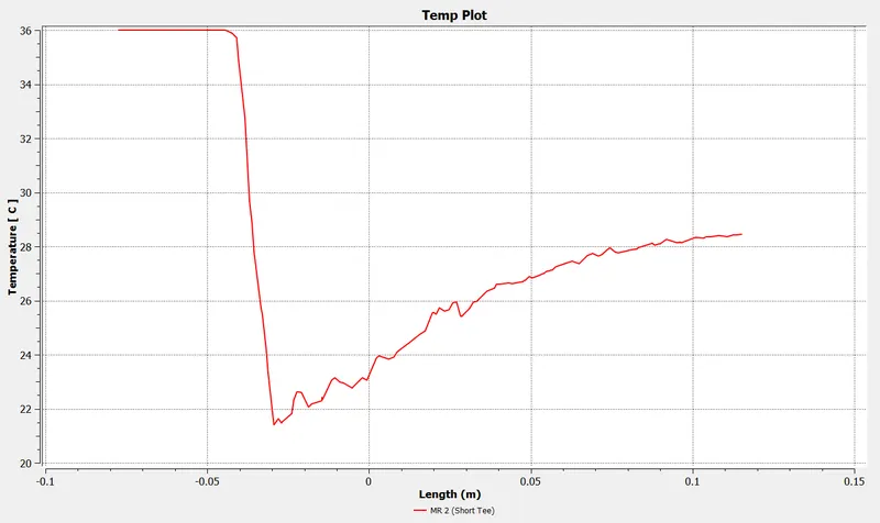



Similarly, a graph 'Velocity Vs Length of the flow' needs to be plotted just by putting the Y variable as 'Velocity'.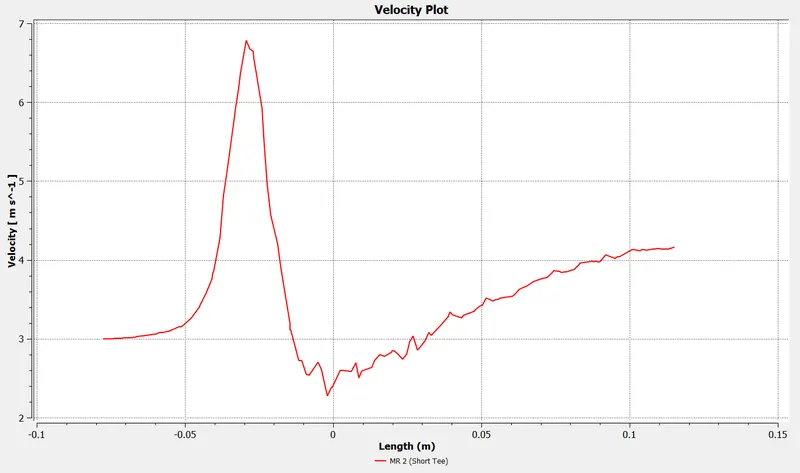



One may export the data generated by the plots to excel to compare the moment ratios of different cases.


For Momentum Ratio = 4 -

In Ansys Workbench, right-click the 'Short Tee - MR 2' system, generate a duplicate copy, and name it 'Short Tee - MR 4'. Now, directly jump into the 'Setup File'.

In Boundary Conditions,

For inlet Y:
We only needed to change the velocity magnitude to 12 m/s from 6 m/s.

Under the Solutions Toolbar, click 'Initialize' choosing the 'Hybrid' method.

We ran the simulation for 200 iterations with the 'Hybrid' method. Here, it got converged at 154 iterations.

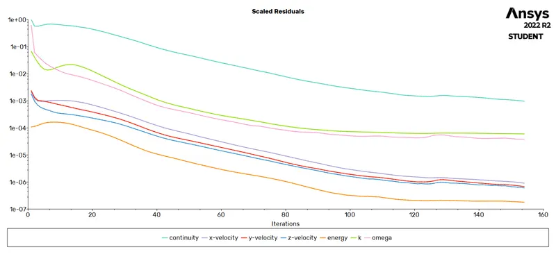
Later, we computed the values of temperature and standard deviation of temperature under the Reports Definitions.

These are the values at the outlet,
Temperature = 27.557621° C
Standard Deviation = 1.0550566° C

Then, we found the minimum, maximum, and average values of velocity and temperature at the outlet.

Velocity:

Average = 6.04097 m/s
Minimum = 4.686356 m/s
Maximum = 6.532316 m/s

Temperature:

Average = 27.56359°C
Minimum = 25.34734°C
Maximum = 29.52029°C

Sr. No.	Parameter	Average	Minimum	Maximum
1.	Temperature (°C)	27.56359	25.34734	29.52029
2.	Velocity (m/sec)	4.686356	6.04097	6.532316

Also, we generated the report.

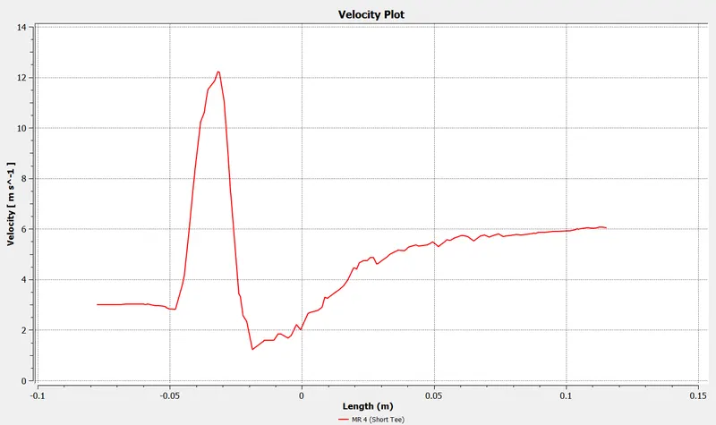
In Post-processing, a 'Temperature Vs Length of the flow' graph was plotted & a 'Velocity Vs Length of the flow' graph was plotted.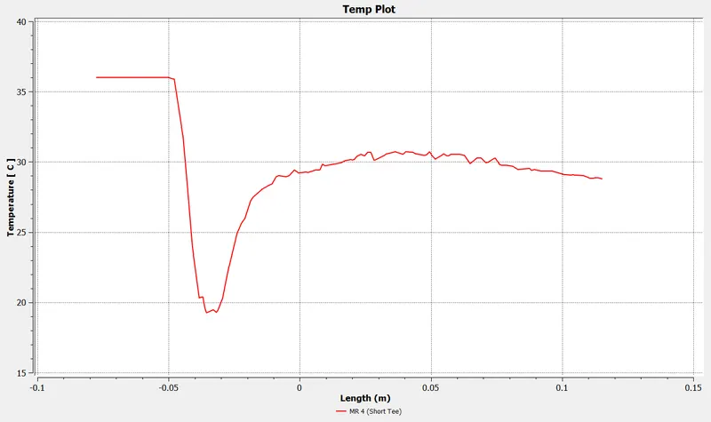

Case 2 - Long Tee Model -

One has to repeat all the steps which were followed in Case 1:

For Momentum Ratio = 2 -

We ran the simulation for 150 iterations with the 'Hybrid' method. Here, it got converged in 126 iterations.

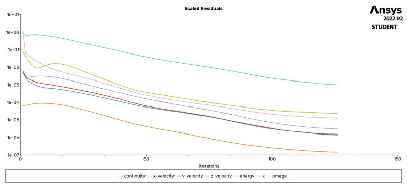
We computed the values of temperature and standard deviation of temperature under the Reports Definitions.

These are the values at the outlet,
Temperature = 30.405494°C
Standard Deviation = 1.0723525°C

We found the minimum, maximum, and average values of velocity and temperature at the outlet.

Velocity:

Average = 4.497539 m/s
Minimum = 2.743969 m/s
Maximum = 4.947217 m/s

Temperature:

Average = 27.56359°C
Minimum = 28.96768°C
Maximum = 33.0332°C

Sr. No.	Parameter	Average	Minimum	Maximum
1.	Temperature (°C)	27.56359	28.96768	33.0332
2.	Velocity (m/sec)	4.497539	2.743969	4.947217

Also, we generated the report.

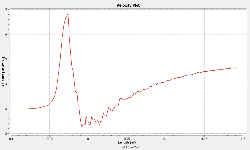
In Post-processing, a 'Temperature Vs Length of the flow' graph was plotted & a 'Velocity Vs Length of the flow' graph was plotted.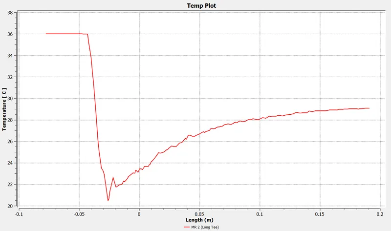

For Momentum Ratio = 4 -

In Ansys Workbench, right-click the 'Long Tee - MR 2' system, generate a duplicate copy, and name it 'Long Tee - MR 4'. Now, directly jump into the 'Setup'.

In Boundary Conditions,

For inlet Y:
We only needed to change the velocity magnitude to 12 m/s from 6 m/s.

Under the Solutions Toolbar, click 'Initialize' choosing the 'Hybrid' method.

We ran the simulation for 250 iterations with the 'Hybrid' method. Here, it got converged at 223 iterations.

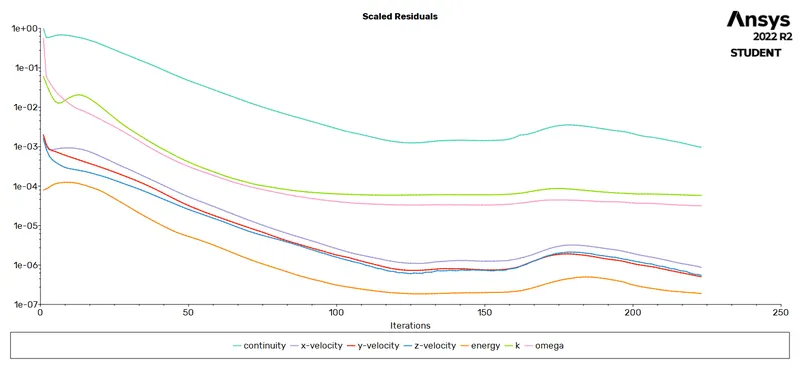
Later, we computed the values of temperature and standard deviation of temperature under the Reports Definitions.

These are the values at the outlet,
Temperature = 27.51645° C
Standard Deviation = 0.58660255° C

Then, we found the minimum, maximum, and average values of velocity and temperature at the outlet.

Velocity:

Average = 6.006118 m/s
Minimum = 4.273362 m/s
Maximum = 6.376619 m/s

Temperature:

Average = 27.54782°C
Minimum = 26.16787°C
Maximum = 28.45846°C

Sr. No.	Parameter	Average	Minimum	Maximum
1.	Temperature (°C)	27.54782	26.16787	28.45846
2.	Velocity (m/sec)	6.006118	4.273362	6.376619

Also, we generated the report.

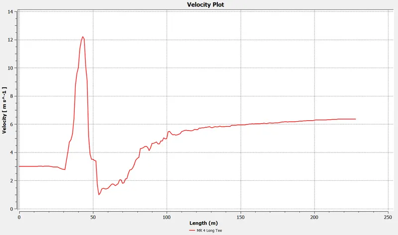
In Post-processing, a 'Temperature Vs Length of the flow' graph was plotted & a 'Velocity Vs Length of the flow' graph was plotted.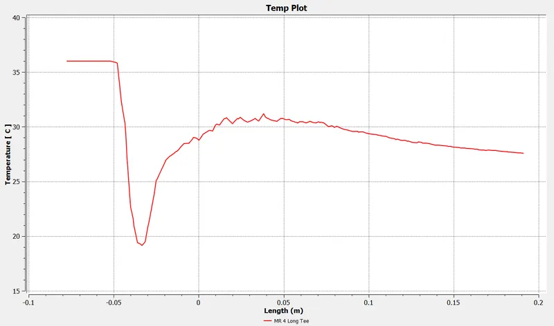





RESULTS -

In the problem statement, it is asked to compare the following values from both cases;

1. Cell count
2. Average outlet temperature
3. Number of iterations for convergence

Sr. No.	Parameters	Case 1 (Short Tee Model)		Case 2 (Long Tee Model)
		MR = 2	MR = 4	MR = 2	MR = 4
1.	Cell Count	69667	69667	69667	69667
2.	Avg. Outlet Temperature (°C)	30.37	27.56	27.56	27.55
3.	No. of Iterations	111	154	126	223

Comparing Temperature Contour Plots:

Temperature Contour Plots Comparison
	Case 1 (Short Tee Model)	Case 2 (Long Tee Model)
MR = 2
MR = 4

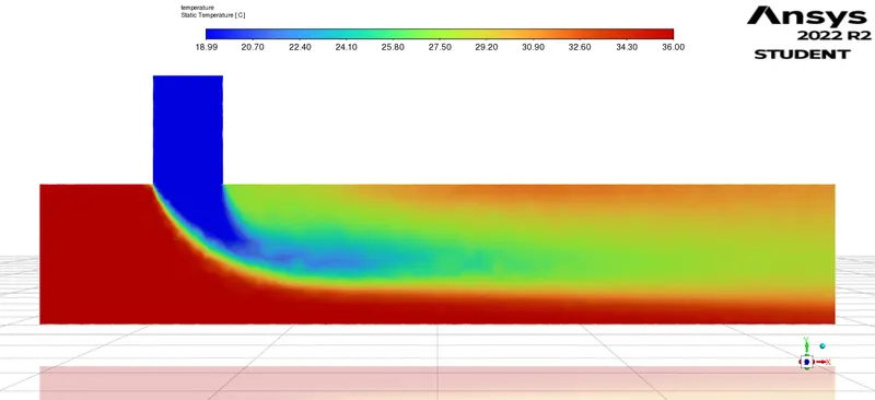
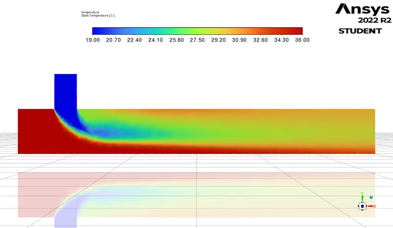
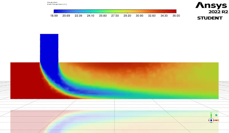
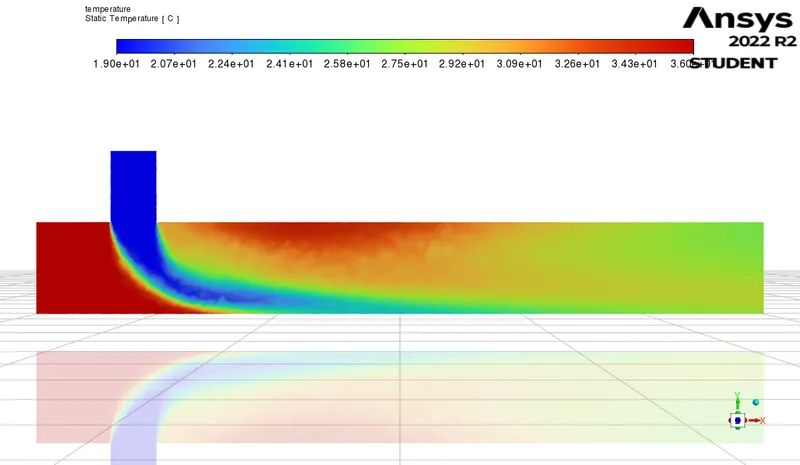
In the case of momentum ratio = 2, it is obvious that no proper fluid mixing has occurred at the pipe's end. In the case of momentum ratio = 4, it can be shown that proper fluid mixing has occurred.

Comparing Velocity Contour Plots:

Velocity Contour Plots Comparison
	Case 1 (Short Tee Model)	Case 2 (Long Tee Model)
MR = 2
MR = 4

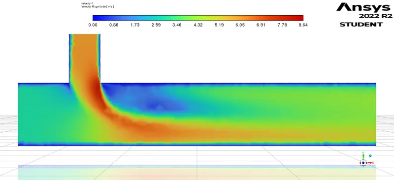
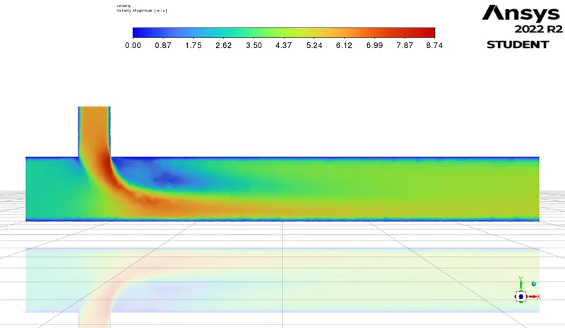
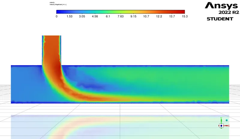
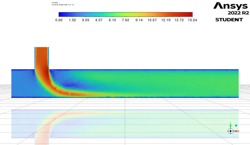
Due to the difference in fluid velocities, a recirculating flow area has developed in both cases. Furthermore, the boundary layer phenomenon is easily seen in each case because the velocity at the pipe wall seen is almost zero. The average velocity at the pipe's end is nearly the same in both cases.

Comparing Temperature Line Plots:

• Short Tee Model with (MR = 2) & Short Tee Model with (MR = 4) -

The final temperature at the outlet for both plots is almost the same. The only difference is that due to the high velocity of cold fluid comparative temperature drop is observed in the plot with MR = 4. As a result, the region of recirculating flow has occurred and temperature at that particular region has increased and sufficient mixing of fluids is observed. While in the plot with MR = 2, no such drastic transition is observed.

• Long Tee Model with (MR = 2) & Long Tee Model with (MR = 4) -

A decent difference is observed in the outlet temperatures for both plots. In the plot with MR = 4, the region of recirculating flow can be observed and the temperature at that particular region has increased. In the plot with MR = 2, this region is not observed. Thus, the best mixing of fluid is observed in the plot with MR = 4.

• Short Tee Model with (MR = 2) & Long Tee Model with (MR = 2) -

The only difference observed between the two plots is that the temperature at the outlet in the plot with the long tee model is slightly more than the short tee model.

• Short Tee Model with (MR = 4) & Long Tee Model with (MR = 4) -

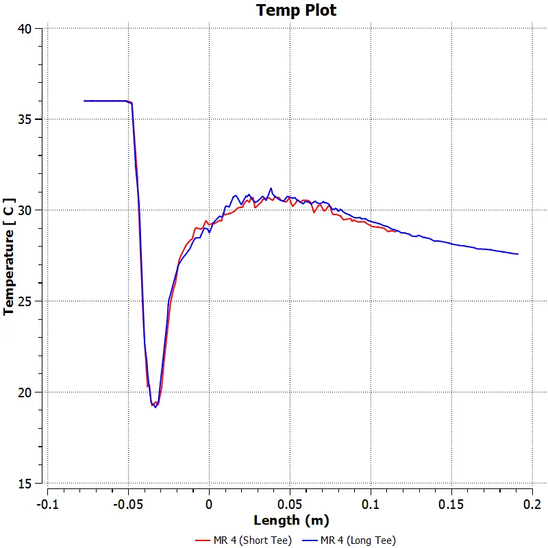
No such difference in the temperature plots is observed. The only difference observed is that the temperature in the long tee model is slightly less than in the short tee model.

Comparing Velocity Line Plots:

In velocity plots, the only observable point is that in plots with MR = 4, the velocity of cold fluid is high while in plots with MR = 2, the velocity of cold fluid is comparatively low. As a result, in former plots, the outlet velocity observed is high and in latter plots, the outlet velocity is low.

CONCLUSION -

As mentioned earlier for better mixing efficiency standard deviation of temperature should be low. Thus, it can be said that - Higher fluid mixing efficiency is achieved when the standard deviation of temperature at the outlet is lower.

Parameter	Case 1 (Short Tee)		Case 2 (Long Tee)
	MR = 2	MR = 4	MR = 2	MR = 4
Standard Deviation of Temperature at the outlet (°C)	1.81	1.06	1.07	0.58

Thus, it can be inferred from the contour plots, line plots, and values of the standard deviation of temperature at the outlet that, the long tee model with momentum ratio = 4 has the highest fluid mixing efficiency. It can also be concluded that the momentum ratio proves dominant over the length of the pipe when we consider the mixing efficiency of fluids in a mixing tee model. Hence, for efficient mixing of fluids in mixing tee models, one should consider the momentum ratio between the fluids first and then the length of the pipe.

If we rank all four models according to how well they mix, it will be -

Long Tee Model (MR 4) > Short Tee Model (MR 4) > Long Tee Model (MR 2) > Short Tee Model (MR 2)

Thus, steady-state simulations were performed for both cases and inferences were derived on the basis of the outcomes obtained.