Week 1- Mixing Tee

Case 1: Short Mixing Tee

Iteration 1: Momentum Ratio-2 (k-epsilon model)

Analytical formula for `T_(mixture)` at outlet:

`T_(mixture)=((m_(hot)**T_(hot))+(m_(cold)**T_(cold)))/(m_(hot)+m_(cold))`

where, m - Mass Flow Rate `=rho**A**v`

`T_(hot)` - Temperature at the cold inlet`=36^oC`

`T_(cold)` - Temperature at the cold inlet`=19^oC`

`T_(mixture)` - Temperature at the outlet

`A_(hot)=901.3138mm^2`

`A_(cold)=225.9823mm^2`

`v_(hot)=3m/s`

`v_(cold)=6m/s`

After calculation, `T_(mixture)=30.322^oC`

Pre-Processing-

Drag and drop the Fluid Flow (Fluent) solver from the right list into the ANSYS Workbench workspace. Ansys Fluent is a general-purpose computational fluid dynamics (CFD) software used to model fluid flow, heat and mass transfer, chemical reactions, and more.

The short mixing tee step model is imported into ANSYS Fluent by right-clicking on the Geometry Cell and selecting import model. Again right clicking on the Geometry Cell and open Spaceclaim which is a multipurpose 3D modeling tool.

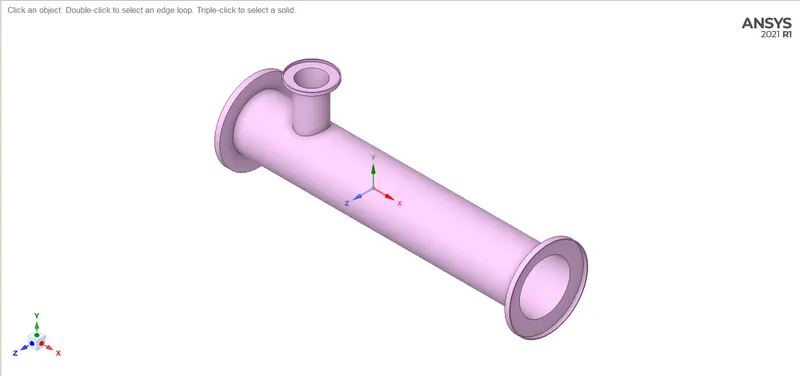
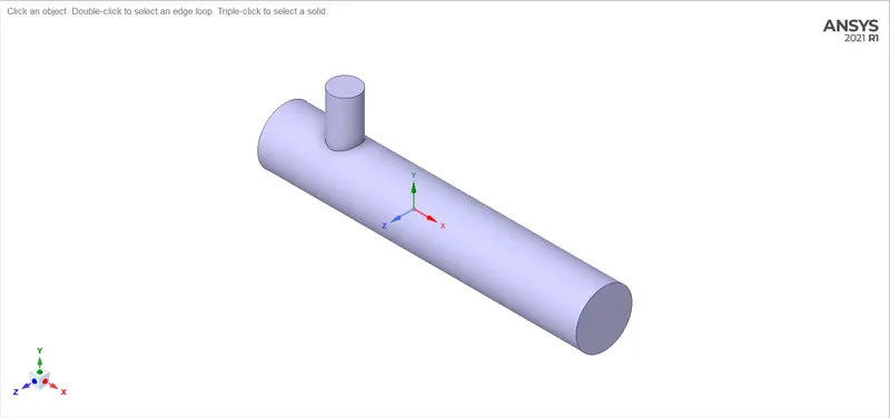
Now, suppressing the outer tee pipe model after extracting volume. Selecting volume extract in the prepare menu for which select three pipe edges and then the green check button.

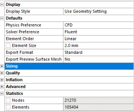
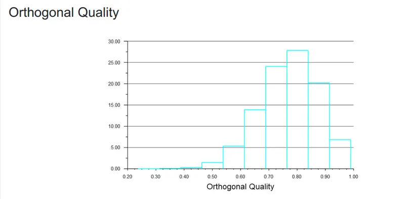
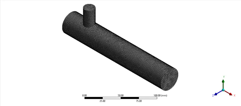
Exiting SpaceClaim and opening Meshing software by double-clicking on the Mesh menu. First, create the named selections for the boundaries by selecting faces: inlet_x, inlet_y, outlet, and wall. Finally, create a mesh with an element size of 2mm and check the mesh using mesh metrics that identify elements according to their quality it can be seen that the elements of low quality are minimal. Most of the elements have very high quality in the range of 0.6 to 1. Hence, the mesh is of acceptable quality.

The meshed model can be seen in the below model:

Solving-

Exiting Mesher, we will need to open Fluent solver by double-clicking on the Setup menu and selecting the parallel mode from the prompted dialog box.

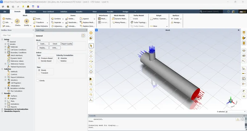
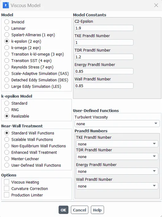
In the outline view, start with General and select pressure-based type in the type, absolute in velocity formulation, and steady state in time under solver. Now, in models select the Energy equation on, and in the viscous select the realizable k-epsilon model for the problem.

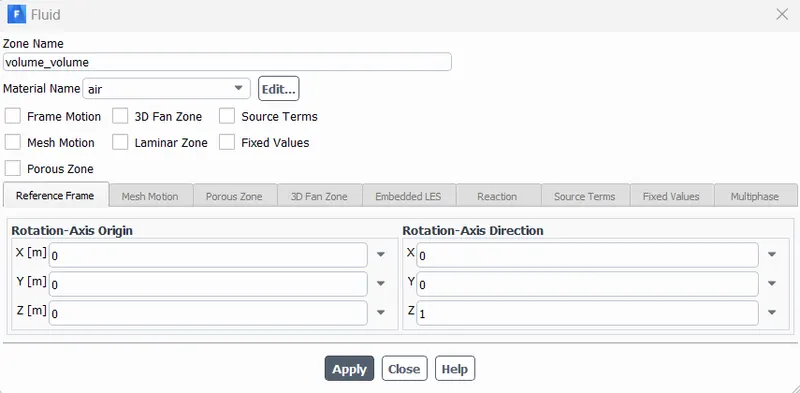
Now, in the Cell Zone Condition checking working fluid material as air is assigned to the volume.

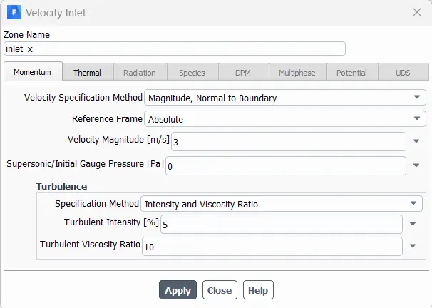
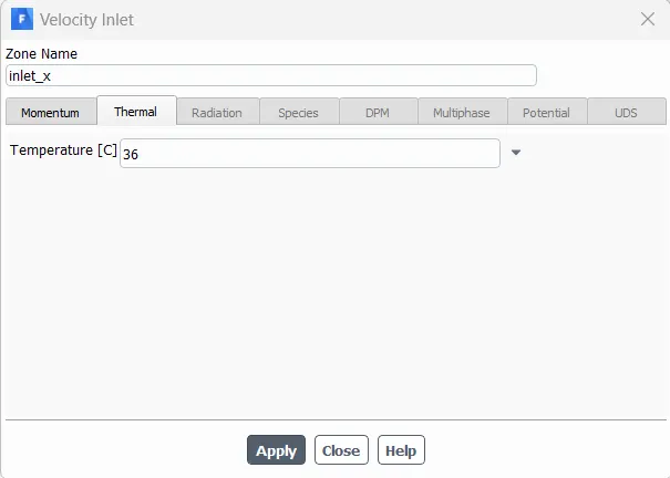
Under Boundary Conditions, select inlet-x and put 3m/s as velocity magnitude and temperature as 36degree celsius for the hot inlet. Similarly for the cold inlet, put 6m/s as velocity magnitude and temperature as 19degree celsius. Changing nothing for the outlet which will be the pressure outlet and for the wall it will be no slip stationary wall.

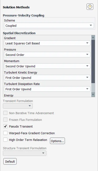
Under Solution, keep default options for methods.

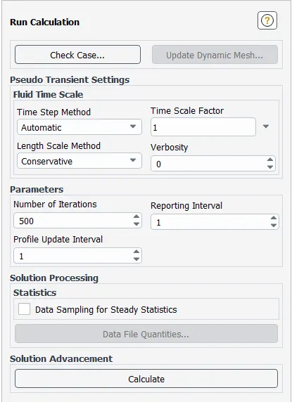
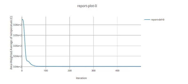
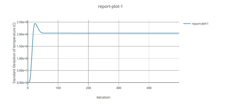
We want to generate a temperature and standard deviation plot report for the outlet which can be set up under Report Definitions. And then select hybrid initialization and initialize the solution which can be found in Initialization. Finally, change the number of iterations to 500 and then select calculate.

Post-Processing-

After completion of the calculation, open the CFD post by double-clicking the Results menu.

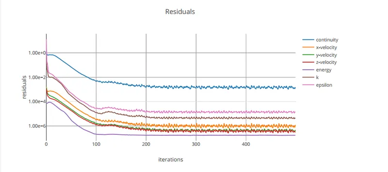
Residual plot:

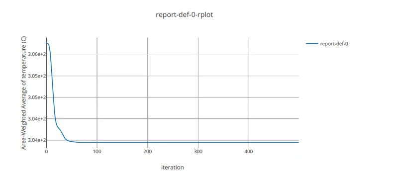
Area-Weighted Temperature plot:

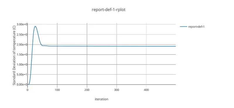
Standard Deviation plot:

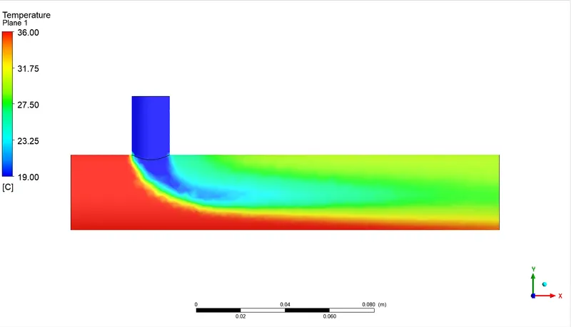
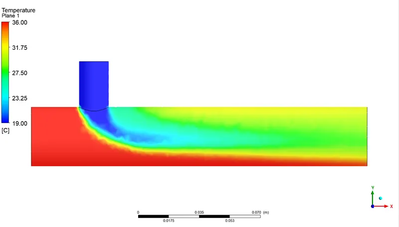
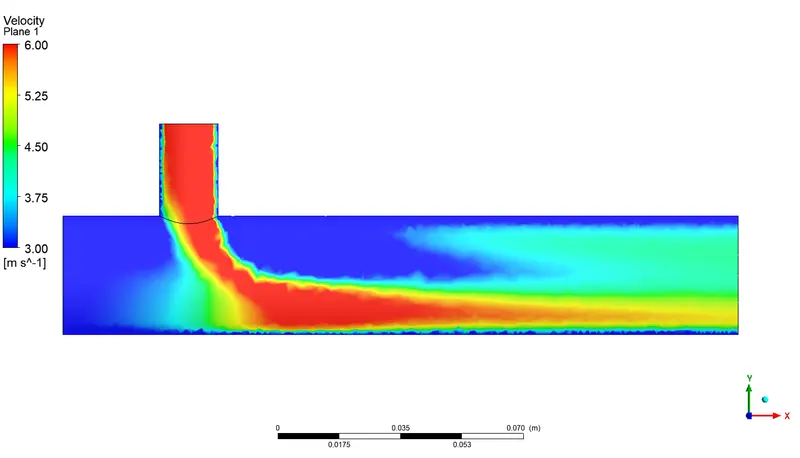
Creating a new plane along XY direction and under the Color menu, selecting temperature and velocity to see contour.

Temperature contour on Plane 1:

Velocity contour on Plane 1:

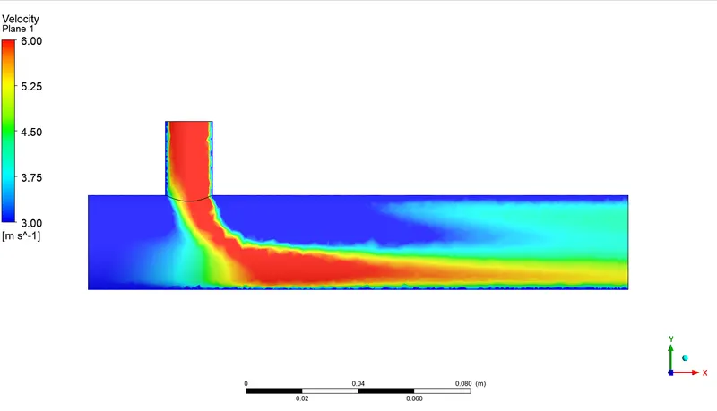
Creating a new plane along the YZ direction and under the Color menu, selecting temperature and velocity to see contour.

Temperature contour on plane 2 at 2D:

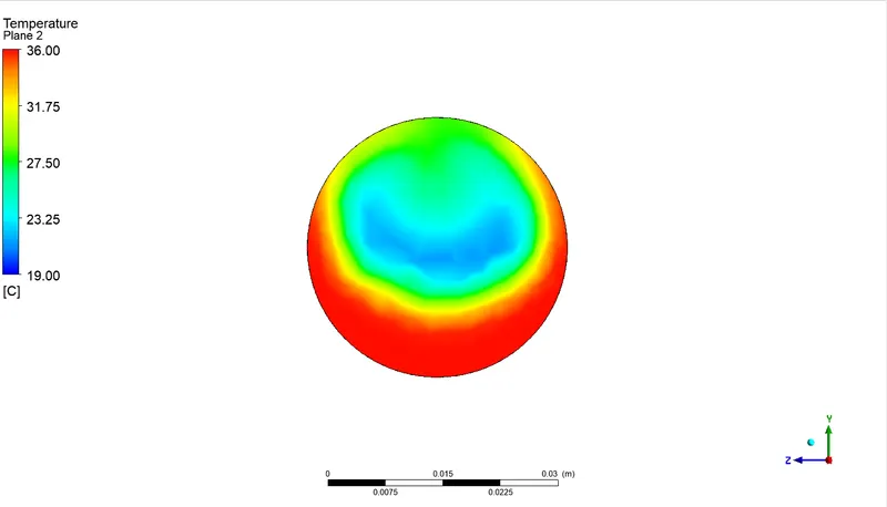
Velocity contour on plane 2 at 2D:

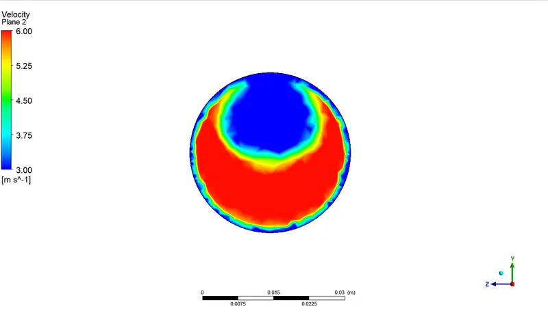
Temperature contour on plane 2 at end of pipe:

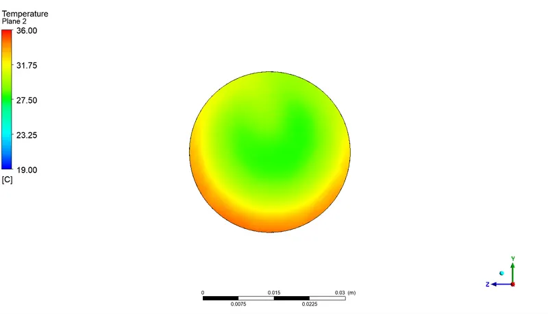
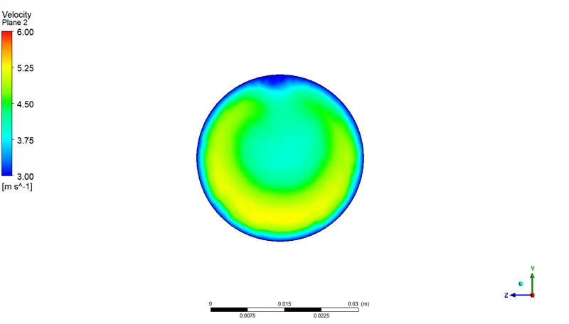
Velocity contour on plane 2 at end of pipe:

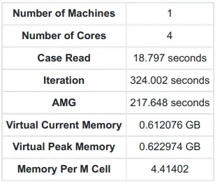
Run information:

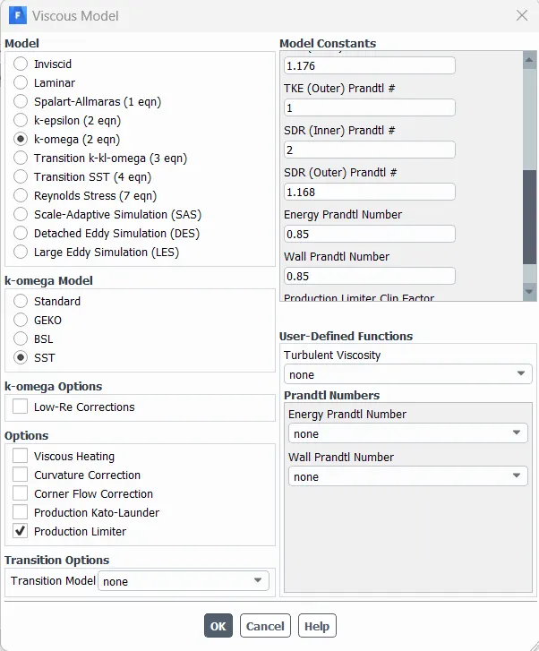
Iteration 2: Momentum Ratio-4 (k-omega model)

Keeping pre-processing data the same and just making changes to Viscous under Models in Fluent by selecting k-omega.

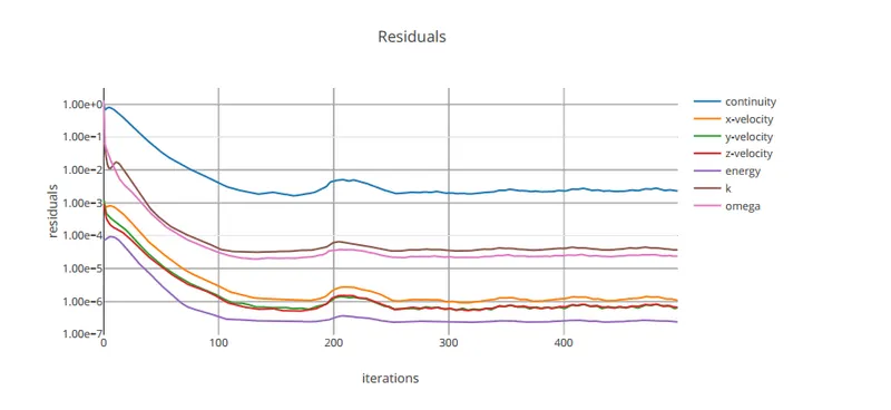
After completion of the calculation, open the CFD post by double-clicking the Results menu.

Residual plot:

Area-Weighted Temperature plot:

Standard Deviation Temperature plot:

Temperature contour on Plane 1:

Velocity contour on Plane 1:

Temperature contour on plane 2 at 2D:

Velocity contour on plane 2 at 2D:

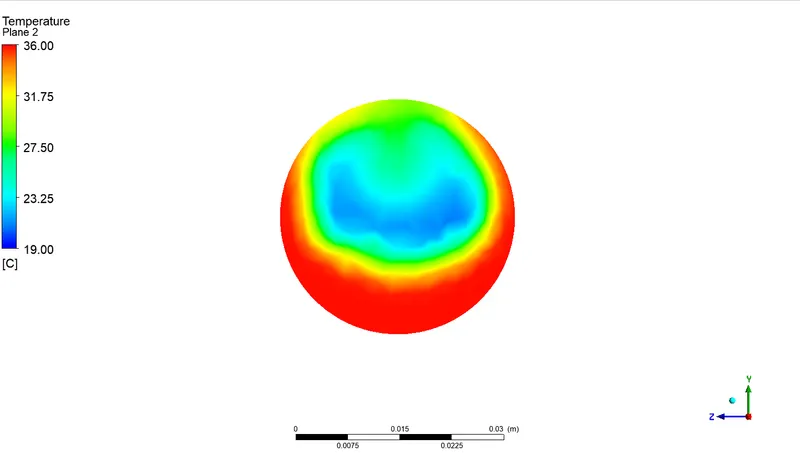
Temperature contour on plane 2 at the end of the pipe:

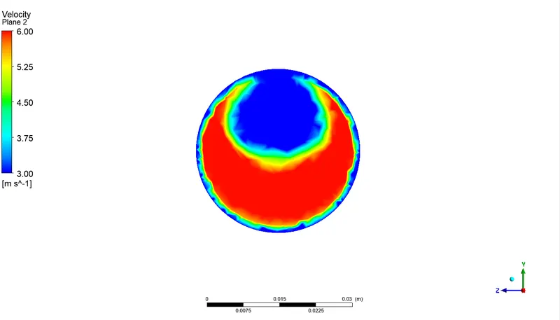
Velocity contour on plane 2 at the end of the pipe:

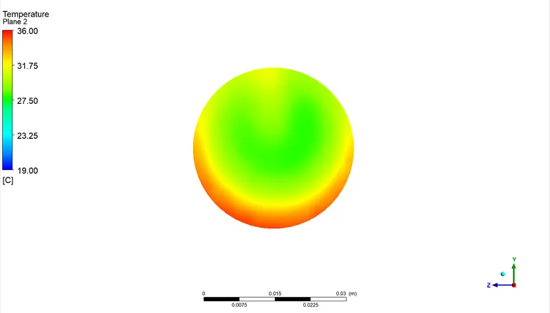
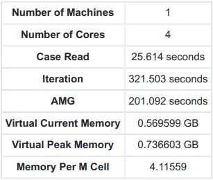
Run information:

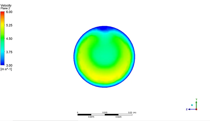
k-epsilon v/s k-omega-

k-epsilon model poorly resolves the viscous layer, unlike the k-omega model. Furthermore, the k-omega model is good at resolving internal flows, separated flows, jets, and flows with high-pressure gradients, and also internal flows through curved geometries. Based on the quick literature review, it seems that the Standard k-epsilon model predicts the flow better than the other turbulence models.

From the residual graph for both k-epsilon and k-omega, it took fewer iterations for k-epsilon to attain convergence. The numerical outlet temperature for k-epsilon is closer to the analytic outlet temperature and also the standard deviation for k-epsilon is less than k-omega. Thus, we will be using the k-epsilon model for the rest of the problems.

Iteration 3- Momentum Ratio-4

Analytical formula for `T_(mixture)` at outlet:

`T_(mixture)=((m_(hot)**T_(hot))+(m_(cold)**T_(cold)))/(m_(hot)+m_(cold))`

where, m - Mass Flow Rate `=rho**A**v`

`T_(hot)` - Temperature at the cold inlet`=36^oC`

`T_(cold)` - Temperature at the cold inlet`=19^oC`

`T_(mixture)` - Temperature at the outlet

`A_(hot)=901.3138mm^2`

`A_(cold)=225.9823mm^2`

`v_(hot)=3m/s`

`v_(cold)=12m/s`

After calculation, `T_(mixture)=27.487^oC`

Keeping pre-processing data the same and just making changes to inlet velocity 12m/s for inlet-y under Boundary Conditions in Fluent.

After completion of the calculation, open the CFD post by double-clicking the Results menu.

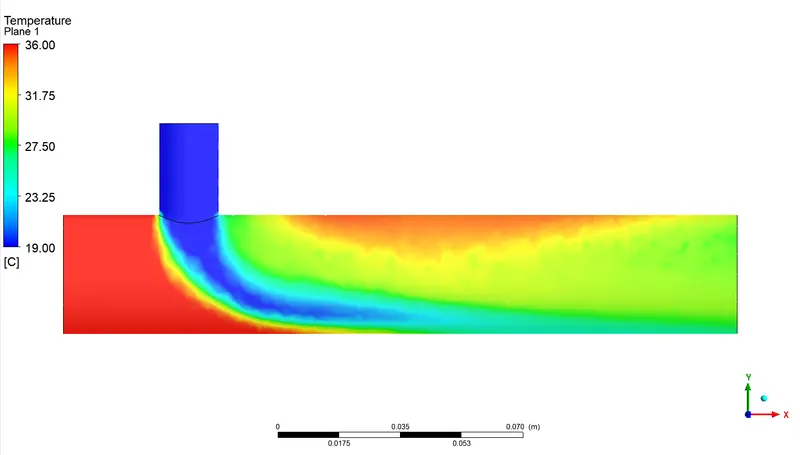
Temperature contour on Plane 1:

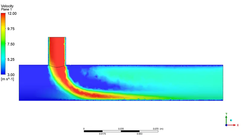
Velocity contour on Plane 1:

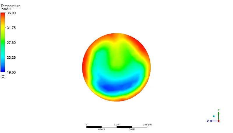
Temperature contour on plane 2 at 2D:

Velocity contour on plane 2 at 2D:

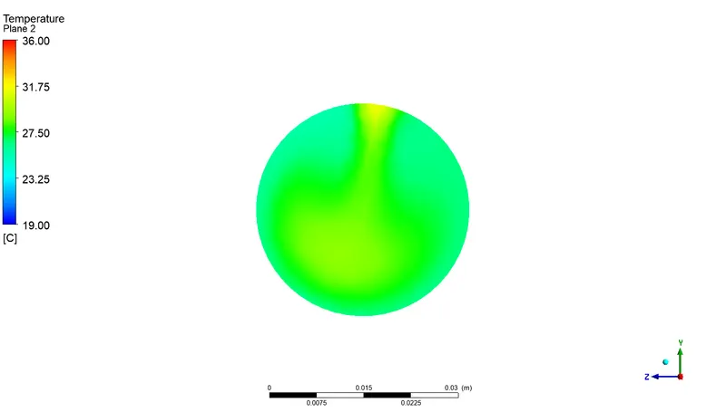
Temperature contour on plane 2 at the end of the pipe:

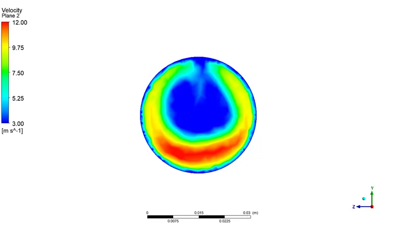
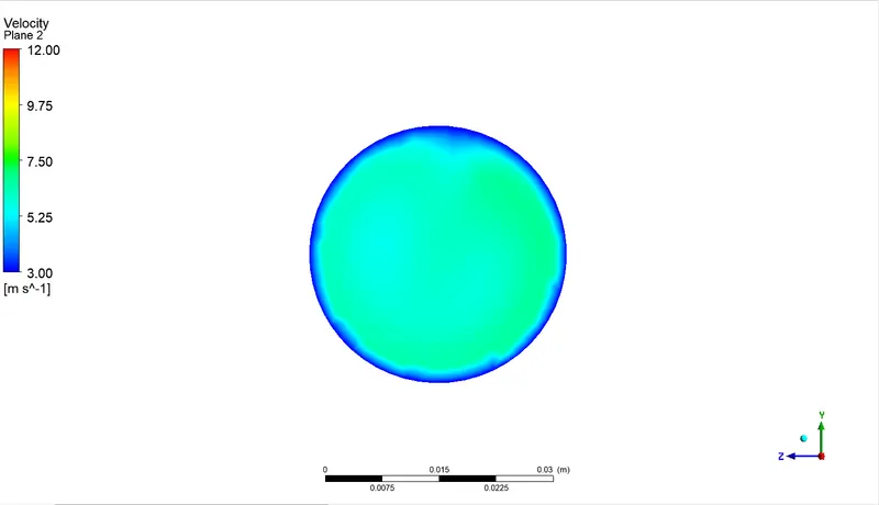
Velocity contour on plane 2 at the end of the pipe:

Case 2: Long Mixing Tee

Iteration 1: Momentum Ratio-2

The short mixing tee step model is imported into ANSYS Fluent by right-clicking on the Geometry Cell and selecting import model. Again right clicking on the Geometry Cell and open Spaceclaim which is a multipurpose 3D modeling tool.

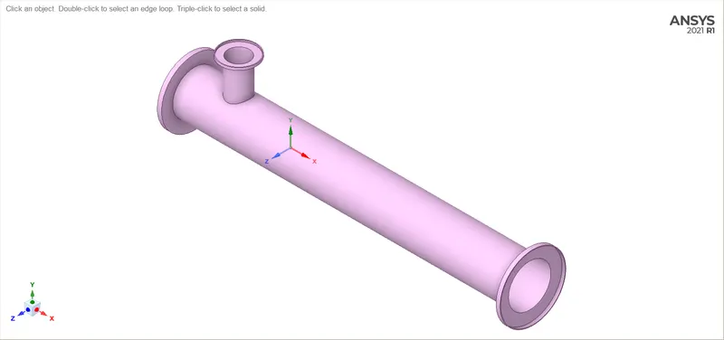
Now, suppressing the outer tee pipe model after extracting volume. Selecting volume extract in the prepare menu for which select three pipe edges and then the green check button.

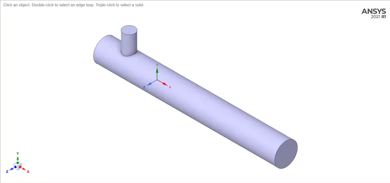
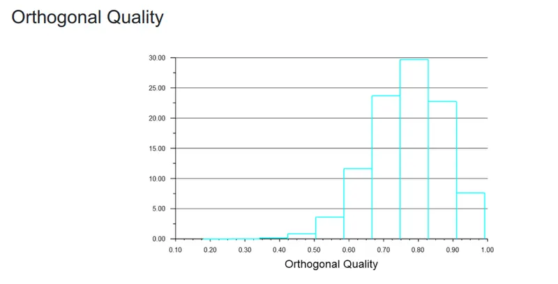
Exiting SpaceClaim and opening Meshing software by double-clicking on the Mesh menu. First, create the named selections for the boundaries by selecting faces: inlet_x, inlet_y, outlet, and wall. Finally, create a mesh with an element size of 2mm and check the mesh using mesh metrics that identify elements according to their quality it can be seen that the elements of low quality are minimal. Most of the elements have very high quality in the range of 0.6 to 1. Hence, the mesh is of acceptable quality.

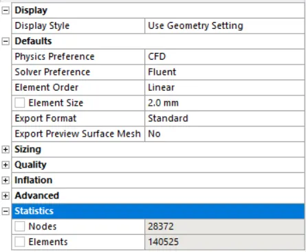
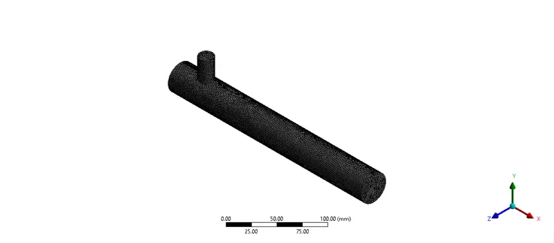
The meshed model can be seen in the below model:

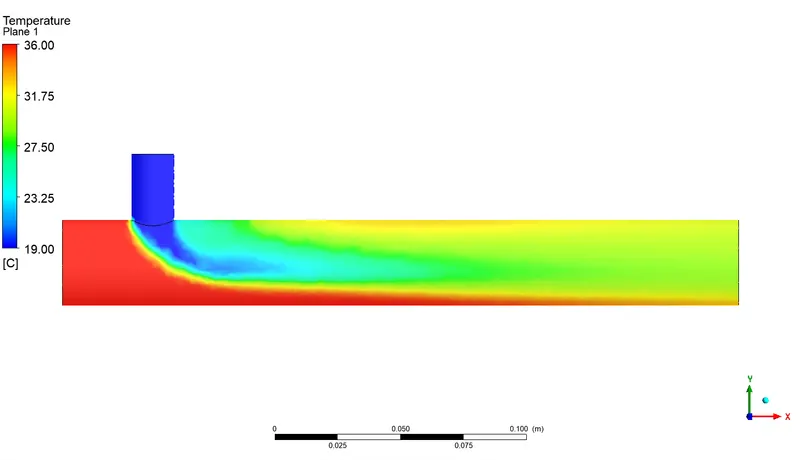
Temperature contour on Plane 1:

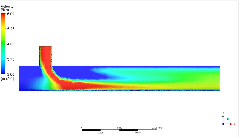
Velocity contour on Plane 1:

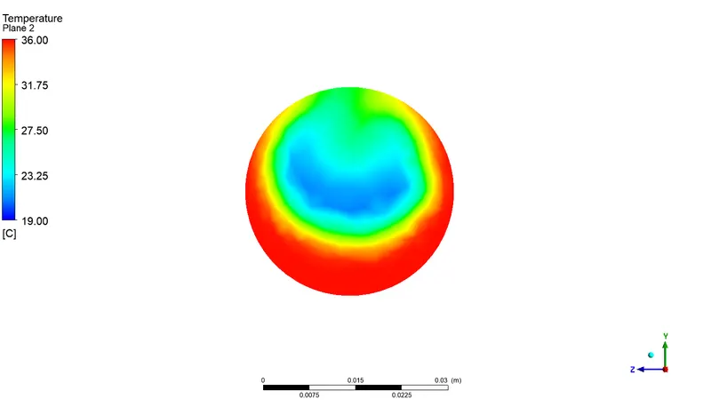
Temperature contour on plane 2 at 2D:

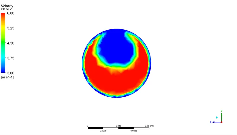
Velocity contour on plane 2 at 2D:

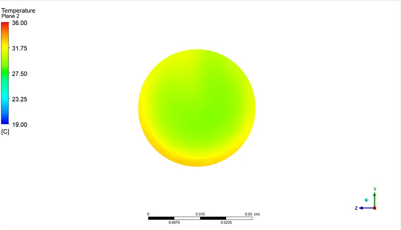
Temperature contour on plane 2 at the end of the pipe:

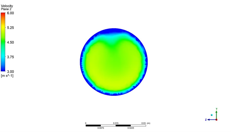
Velocity contour on plane 2 at the end of the pipe:

Iteration 2: Momentum Ratio-4

Keeping pre-processing data the same and just making changes to inlet velocity 12m/s for inlet-y under Boundary Conditions in Fluent.

After completion of the calculation, open the CFD post by double-clicking the Results menu.

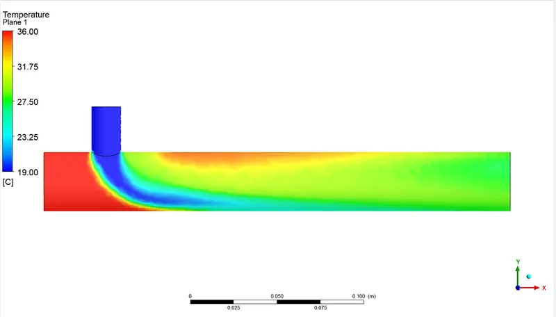
Temperature contour on Plane 1:

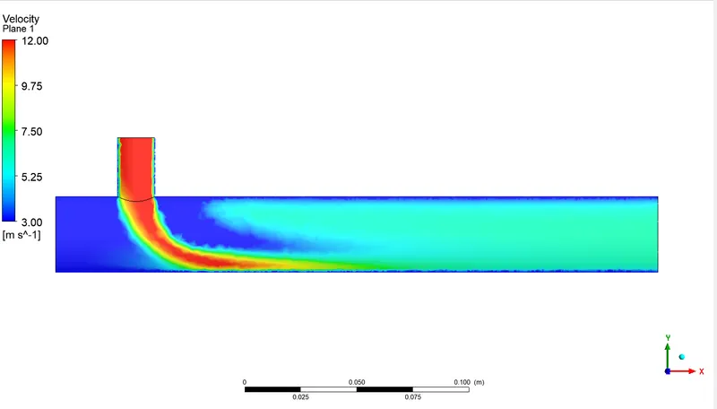
Velocity contour on Plane 1:

Temperature contour on plane 2 at 2D:

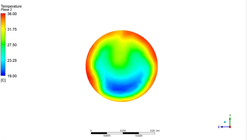
Velocity contour on plane 2 at 2D:

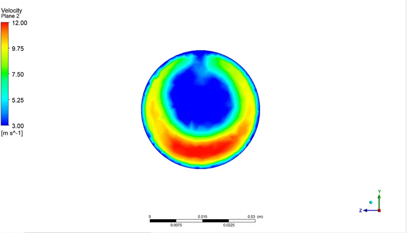
Temperature contour on plane 2 at the end of the pipe:

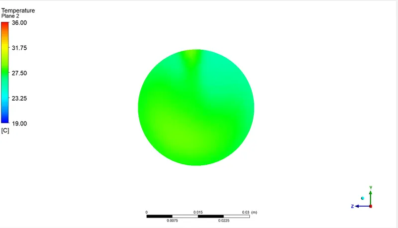
Velocity contour on plane 2 at the end of the pipe:

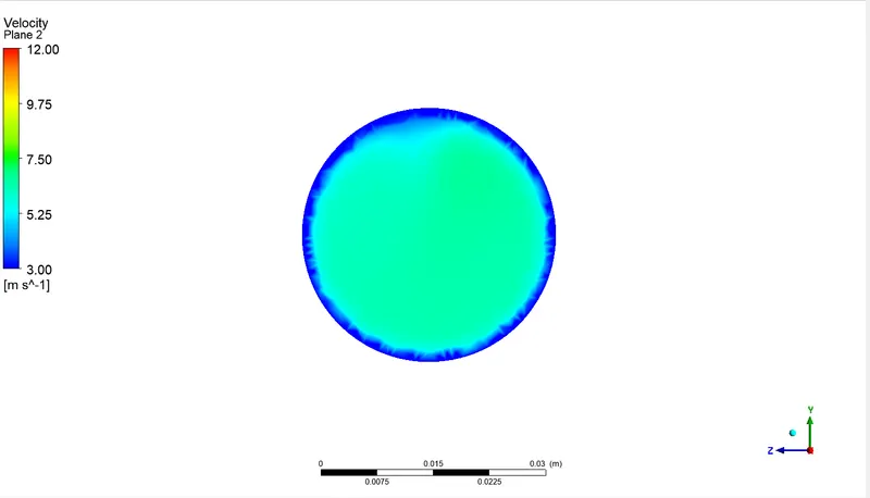
Mesh Independence test - Case 1 Iteration 1

A mesh independence study is a method of investigating, whether the simulation results are independent of the underlying mesh or not. You do it by running a few simulations with different mesh resolutions and checking if the results change.

Sr. No.	Element Size	No of Cells	Iteration time	Temperature	Standard Deviation
1	1mm	531403	382.21sec	30.4021C	1.9174C
2	2mm	105404	310.47sec	30.2949C	1.9083C
3	3mm	39803	119.12sec	30.2053C	2.0668C
4	4mm	21977	68.89sec	30.2236C	1.8060C
5	5mm	14330	43.54sec	30.2799C	1.1197C

• From the above table, we can say that our mesh is independent which means there are no large changes in outlet temperature by increasing the number of elements.
• So we can prefer less number of elements mesh also for simulations. For element sizes of 2mm and 4mm it is close to the analytical temperature.
• For a 1mm element size, we can say that it is too fine and does not give accurate results. Smaller mesh size is used where large deformation is anticipated because of local buckling, i.e. at the welded joint of two sections with different thicknesses and at the base of the pier.
• It can also be seen that computational iteration time exponentially decreases as we increase element size.

Effect of length and momentum ratio on results -

Sr. No.	Type	Momentum ratio	Analytic Temperature	Numerical Temperature	Error	Numerical Standard Deviation	Iteration Time
1	Short Tee	2	30.322C	30.2949C	0.0271C	1.9083C	310.473sec
2	Short Tee	4	27.487C	27.5405C	-0.0535C	0.9705C	330.902sec
3	Long Tee	2	30.322C	30.4286C	-0.1066C	1.0356C	317.986sec
4	Long Tee	4	27.487C	27.5005C	-0.0135C	0.7394C	421.024sec

• From the above results, we can say that the outlet temperature is independent of the length of the mixing tee.
• The momentum ratio affects the outlet temperature. By increasing the momentum ratio outlet temperature is dropping. Also, computational iteration time increases with MR.
• From the above validation of numerical and analytical values, we can say that numerical simulation values are matching with analytical values.
• Now, comparing MR 2 & 4, for both long and short TEE the computational time taken for MR 4 is large even though no. of elements is the same.
• Comparing Long & Short Tee for the same MR, with longer TEE is more efficient and preferable for MR of 4 and vice-versa.