Week 7 - Simulation of a 1D Super-sonic nozzle flow simulation using Macormack Method

Consider an isentropic flow through a convergent-divergent nozzle with length L or x .

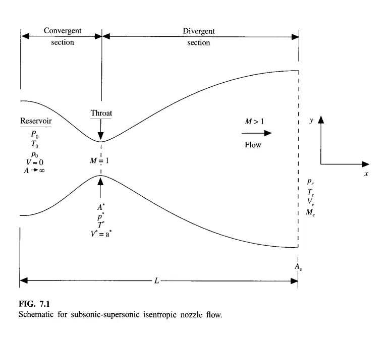
The area at the opening is very large , hence the velocity is considered to be very small (approximately 0) . The velocity increases as it passes through the nozzle and exits at supersonic speed . The area is minimum at throat and here velocity is considered to be equal to speed of sound (M=1) . Here the sectional area varies as a function of distance x . Here we consider that the variables vary along x direction only . Hence we consider this as a quasi-one-dimensional flow . The pressure difference at inlet and outlet leads to the increase in velocity .

Given below are the governing equations for quasi-one -dimesional flow .

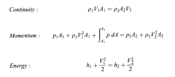
Conservative form of above governing equations-

Continuity:

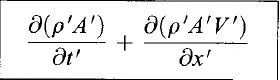
Momentum:

Energy:

Non conservative form of above governing equations -

Continuity:

Momentum:

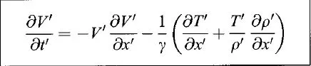
Energy:

The difference between the conservative and non-conservative form of governing equation is that both forms give the same analytical solution but the different numerical output. Conservative form provides accurate results and it can provide better results in the presence of shocks or discontinuities.

Main Code-

clear all
close all
clc

L = 3; %domain length
n = [31 62 93]; %grid points
CFL = 0.5;

th = (n-1)/2; %throat position
nt = 1:1400;

for i  = 1:length(n)
    x = linspace(0, L, n(i));
    [m_NC, m_th_NC] = non_conservative(L, n(i), nt, CFL);
    [m_C, m_th_C] = conservative(L, n(i), nt, CFL);
    
    figure(7)
    tiledlayout(2,1)
    nexttile
    plot(nt, m_th_NC, 'b', nt, m_th_C, 'r', 'linewidth', 1)
    xlabel('Time steps')
    ylabel('Mass flow rate')
    legend('Conservative form','Non-Conservative form')
    title('Mass flow rate at throat point')
    
    nexttile
    plot(x, m_C, 'b', x, m_NC, 'r', 'linewidth', 1)
    xlabel('Length of nozzle')
    ylabel('Mass flow rate')
    legend('Conservative form','Non-Conservative form')
    title('Mass flow rate at nozzle')
    
    figure(8)
    tiledlayout(2,1)
    nexttile
    plot(nt, m_th_C, 'linewidth', 1)
    hold on
    xlabel('Time steps')
    ylabel('Mass flow rate')
    legend('n = 31 nodes','n = 62 nodes','n = 93 nodes')
    title('Grid independency test (Conservative form) at throat')
    
    nexttile
    plot(nt,m_th_NC,'linewidth',1)
    hold on
    xlabel('Time steps')
    ylabel('Mass flow rate')
    legend('n = 31 nodes','n = 62 nodes','n = 93 nodes')
    title('Grid independency test (Non-Conservative form) at throat')
    
    figure(9)
    tiledlayout(2,1)
    nexttile
    plot(x, m_C, 'linewidth',1)
    hold on
    xlabel('Length of nozzle')
    ylabel('Mass flow rate')
    legend('n = 31 nodes','n = 62 nodes','n = 93 nodes')
    title('Grid independency test (Conservative) along the nozzle')

    nexttile
    plot(x,m_NC,'linewidth',1)
    hold on
    xlabel('Length of nozzle')
    ylabel('Mass flow rate')
    legend('n = 31 nodes','n = 62 nodes','n = 93 nodes')
    title('Grid independency test (Non-Conservative) along the nozzle')
end

Function Code for Non-Conservative form

function [m_NC, m_th_NC] = non_conservative(L,n,nt,CFL)
x = linspace(0,L,n);
dx = x(2)-x(1);

rho = 1 - 0.3146*x;
T = 1 - 0.2314*x;
V = (0.1 + 1.09*x).*T.^0.5;
A = 1 + (2.2*(x-1.5).^2); %area
gamma = 1.4; %speific heat at constant pressure


M = V./(T.^0.5);
m = rho.*A.*V;
P = rho.*T;

for ii = 1:n
    u = (T(ii))^0.5;
    dt(ii) = CFL*dx/(u + V(ii));
end
dt = min(dt);

for i = 1:length(nt)
    % initial values    
    rho_old = rho;
    T_old = T;
    V_old = V;
    
        for j = 2:n-1
            %predictor step
            drho_dx = (rho(j+1)-rho(j))/dx;
            dV_dx = (V(j+1)-V(j))/dx;
            dT_dx = (T(j+1)-T(j))/dx;
            dA_dx = (log(A(j+1))-log(A(j)))/dx;
        
            drho_dt_p(j) = -rho(j)*dV_dx - rho(j)*V(j)*dA_dx - V(j)*drho_dx;
            dV_dt_p(j) = -V(j)*dV_dx - (1/gamma)*(dT_dx + (T(j)/rho(j))*drho_dx);
            dT_dt_p(j) = -V(j)*dT_dx - (gamma-1)*T(j)*(dV_dx + V(j)*dA_dx);
        
            %updating primitives
            V(j) = V_old(j) + dV_dt_p(j)*dt;
            rho(j) = rho_old(j) + drho_dt_p(j)*dt;
            T(j) = T_old(j) + dT_dt_p(j)*dt;
        
            %corrector step
            drho_dx = (rho(j)-rho(j-1))/dx;
            dV_dx = (V(j)-V(j-1))/dx;
            dT_dx = (T(j)-T(j-1))/dx;
            dA_dx = (log(A(j))-log(A(j-1)))/dx; 
        
            drho_dt_c(j) = -rho(j)*dV_dx - rho(j)*V(j)*dA_dx - V(j)*drho_dx; %continuity    
            dV_dt_c(j) = -V(j)*dV_dx - (1/gamma)*(dT_dx + (T(j)/rho(j))*drho_dx); %momentum
            dT_dt_c(j) = -V(j)*dT_dx - (gamma-1)*T(j)*(dV_dx + V(j)*dA_dx); %energy
        end
    
        %average time derivatives
        drho_dt_avg = 0.5*(drho_dt_p + drho_dt_c);
        dV_dt_avg = 0.5*(dV_dt_p + dV_dt_c);
        dT_dt_avg = 0.5*(dT_dt_p + dT_dt_c);
    
        for k = 2:n-1
            rho(k) = rho_old(k) + drho_dt_avg(k)*dt;
            V(k) = V_old(k) + dV_dt_avg(k)*dt;
            T(k) = T_old(k) + dT_dt_avg(k)*dt;
        end
        
        % entry BC
        V(1) = 2*V(2) - V(3);
        
        % exit BC
        V(n) = 2*V(n-1) - V(n-2);
        rho(n) = 2*rho(n-1) - rho(n-2);
        T(n) = 2*T(n-1) - T(n-2);
        
        % final primitive update
        P = rho.*T;
        M = V./T.^0.5;
        error(k) = abs(V(k) - V(k-1));
        m = rho.*A.*V;
    
        T_th(i) = T(16);
        rho_th(i) = rho(16);
        V_th(i) = V(16);
        M_th(i) = M(16);
        P_th(i) = P(16);
        error_th(i) = error(16);
        m_th(i) = m(16);
        
        if n == 31
            for ij = [1:50:201 700]
                if ij == i
                figure(1)
                plot(x, m, 'linewidth', 1)
                hold on
                title('Variation of mass flow rate at different time steps (Non Conservative)')
                xlabel('Length alongside Nozzle')
                ylabel('Mass Flow Rate')
                elseif i==1400
                plot(x, m, '*r')
                legend('dt = 1', 'dt = 51', 'dt = 101', 'dt = 151', 'dt = 201', 'dt = 700', 'dt = 1400')
                end
            end
        end
end
  

if n == 31
    figure(2)
    plot(x, V, 'b', x, P, 'r', x, T, 'k', x, rho, 'm', x, M, 'g', x, m, 'c')
    ylim([-0.1 3.7])
    title(sprintf('Time step = %d', i))
    xlabel('Length alongside Nozzle')
    ylabel('Non-Dimensional Parameters')
    legend('Velocity', 'Pressure', 'Temperature', 'Density', 'Mach Number', 'Mass Flow Rate')
    title('Steady-State distribution of primitive variables (Non-Conservative)')
    
    figure(3)
    plot(nt, rho_th)
    hold on
    plot(nt, V_th, 'linewidth', 1)
    plot(nt, P_th, 'linewidth', 1)
    plot(nt, T_th, 'linewidth', 1)
    plot(nt, M_th, 'linewidth', 1)
    plot(nt, m_th, 'linewidth', 1)
    xlabel('Time Steps')
    ylabel('Non-Dimensional Parameters')
    legend('Density', 'Velocity', 'Pressure', 'Temperature', 'Mach Number', 'Mass Flow Rate')
    title('Time-wise variation of the primitive variables at throat')
end

m_NC = m;
m_th_NC = m_th;
end

Function Code for Conservative form-

function [m_C, m_th_C] = conservative(L, n, nt, CFL)

x = linspace(0, L, n);
dx = x(2) - x (1);

for ji = length(x)
    if (x(ji)<=0.5)
        rho(ji) = 1;
        T(ji) = 1;
    elseif (x(ji)>0.5) && (x(ji)<=1.5)
        rho(ji) = 1 - 0.366*(x(ji) - 0.5);
        T(ji) = 1 - 0.167*(x(ji) - 0.5);
    else
        rho(ji) = 0.634 - 0.3879*(x(ji) - 1.5);
        T(ji) = 0.833 - 0.3507*(x(ji) - 1.5);
    end
end

A = 1 + (2.2*(x - 1.5).^2); %area
V = 0.59./(rho.*A);
gamma = 1.4; %speific heat at constant pressure

% solution vectors
u1 = rho.*A;
u2 = rho.*A.*V;
u3 = rho.*A.*((T./(gamma-1)) + (gamma-2).*V.^2);

M = V./(T.^0.5); %mach number
m = rho.*A.*V; %mass flow rate
P = rho.*T; %pressure

for jj = 1:31
    u = (T(jj)^0.5);
    dt(jj) = CFL*dx/(u + V(jj));
end
dt = min(dt);

for i = 1:length(nt)
    % initial values
    u1_old = u1;
    u2_old = u2;
    u3_old = u3;
    
    % flux terms
    f1 = u2;
    f2 = ((u2.^2)./u1)+((gamma-1)/gamma)*(u3-((gamma-2)*(u2.^2)./u1));
    f3 = ((gamma.*u2.*u3)./u1)-((gamma*(gamma-1)/2)*(u2.^3)./(u1.^2));
    
    for j = 2:n-1
        
        % source term for predictor step
        s1(j) = (1/gamma)*rho(j)*T(j)*((A(j+1)-A(j))/dx);
        
        % predictor step 
        du1_dt_p(j) = -(f1(j+1)-f1(j))/dx; % continuity
        du2_dt_p(j) = -(f2(j+1)-f2(j))/dx + s1(j); % momentum
        du3_dt_p(j) = -(f3(j+1)-f3(j))/dx; % energy
        
        % updating solution vectors
        u1(j) = u1_old(j) + du1_dt_p(j)*dt;
        u2(j) = u2_old(j) + du2_dt_p(j)*dt;
        u3(j) = u3_old(j) + du3_dt_p(j)*dt;
    
        % updating primitives
        rho = u1./A;
        V = u2./u1;
        T = (gamma-1).*(u3./u1-(gamma-2).*(u./u1).^2);
        
        % updating flux terms
        f1 = u2;
        f2 = ((u2.^2)./u1)+((gamma-1)/gamma)*(u3-((gamma-2)*(u2.^2)./u1));
        f3 = ((gamma.*u2.*u3)./u1)-((gamma*(gamma-1)/2)*(u2.^3)./(u1.^2));
        
        % source term for continuity step
        s2(j) = (1/gamma)*rho(j)*T(j)*((A(j+1)-A(j))/dx);
        
        % corrector step
        du1_dt_c(j) = -(f1(j)-f1(j-1))/dx;
        du2_dt_c(j) = -(f2(j)-f2(j-1))/dx + s2(j);
        du3_dt_c(j) = -(f3(j)-f3(j-1))/dx;
    end
    
    du1_dt_avg = 0.5*(du1_dt_p + du1_dt_c);
    du2_dt_avg = 0.5*(du2_dt_p + du2_dt_c);
    du3_dt_avg = 0.5*(du3_dt_p + du3_dt_c);
    
    for k = 2:n-1
        u1(k) = u1_old(k) + du1_dt_avg(k)*dt;
        u2(k) = u2_old(k) + du2_dt_avg(k)*dt;
        u3(k) = u3_old(k) + du3_dt_avg(k)*dt;
    end
    
    % entry BC
    u1(1) = rho(1)*A(1);
    u2(1) = 2*u2(2) - u2(3);
    u3(1) = u1(1)*(T(1)/(gamma-1) + (gamma/2)*V(1)^2);
    
    % exit BC
    u1(n) = 2*u1(n-1) - u1(n-2);
    u2(n) = 2*u2(n-1) - u2(n-2);
    u3(n) = 2*u3(n-1) - u3(n-2);
    
    % final primitive update
    rho = u1./A;
    V = u2./u1;
    T = (gamma-1).*(u./u1-(gamma/2).*(u2./u1).^2);
    P = rho.*T;
    M = V./T.^0.5;
    error(k) = abs(V(k)-V(k-1));
    m = u2;
    
    T_th(i) = T(16);
    rho_th(i) = rho(16);
    V_th(i) = V(16);
    M_th(i) = M(16);
    P_th(i) = P(16);
    error_th(i) = error(16);
    m_th(i) = m(16);
    
    if n == 31
            for jk = [1:50:201 700]
                if jk == i
                figure(4)
                plot(x, m, 'linewidth', 1)
                hold on
                title('Variation of mass flow rate at different time steps (Conservative)')
                xlabel('Length alongside Nozzle')
                ylabel('Mass Flow Rate')
                elseif i == 1400
                plot(x, m, '*r')
                legend('dt = 1', 'dt = 51', 'dt = 101', 'dt = 151', 'dt = 201', 'dt = 700', 'dt = 1400')
                end
            end
    end
end
  

if n == 31
    figure(5)
    plot(x, V, 'b', x, P, 'r', x, T, 'k', x, rho, 'm', x, M, 'g', x, m, 'c')
    ylim([-0.1 3.7])
    title(sprintf('Time step = %d', i))
    xlabel('Length alongside Nozzle')
    ylabel('Non-Dimensional Parameters')
    legend('Velocity', 'Pressure', 'Temperature', 'Density', 'Mach Number', 'Mass Flow Rate')
    title('Steady-State distribution of primitive variables (Conservative)')
    
    figure(6)
    plot(nt, rho_th)
    hold on
    plot(nt, V_th, 'linewidth', 1)
    plot(nt, P_th, 'linewidth', 1)
    plot(nt, T_th, 'linewidth', 1)
    plot(nt, M_th, 'linewidth', 1)
    plot(nt, m_th, 'linewidth', 1)
    xlabel('Time Steps')
    ylabel('Non-Dimensional Parameters')
    legend('Density', 'Velocity', 'Pressure', 'Temperature', 'Mach Number', 'Mass Flow Rate')
    title('Time-wise variation of the primitive variables at throat (Conservative)')
end

m_C = m;
m_th_C = m_th;
end

Results-

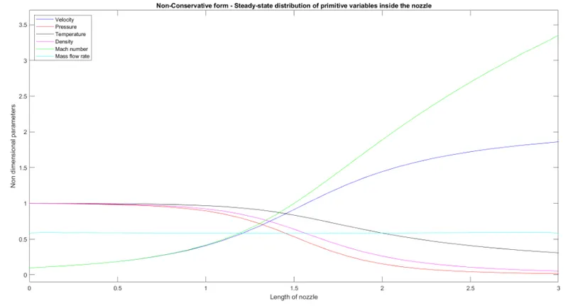
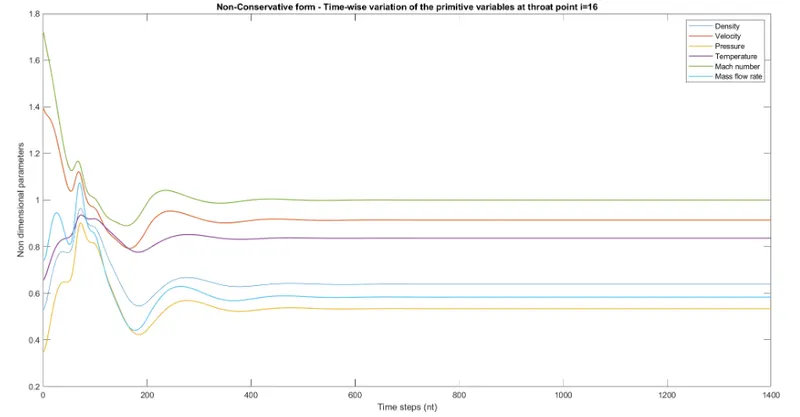
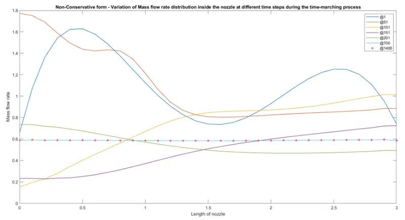
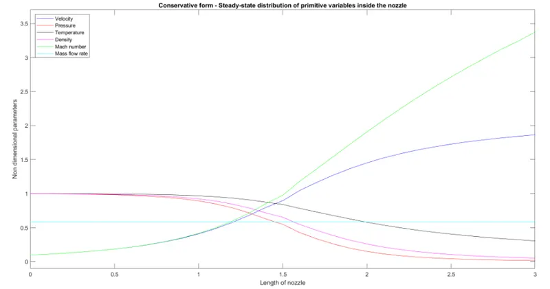
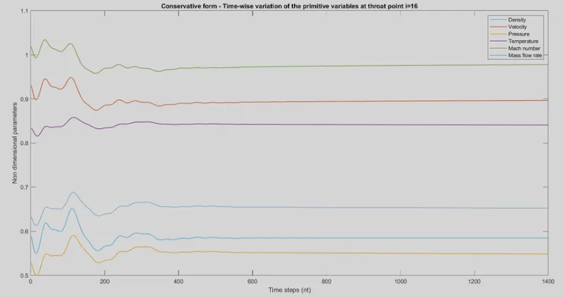
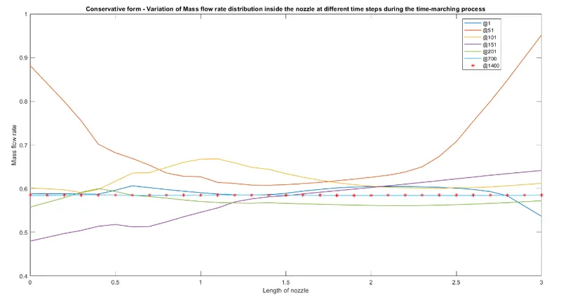
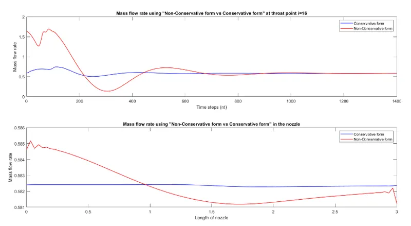
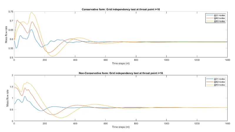
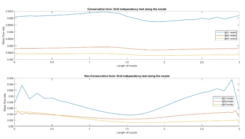
Conclusion -

Grid dependency is an important factor to determine whether the problem can be solved faster. So here we increased the Grid points from 31 to 61 and populated them in a sheet.I t is clear from the above table that the values are almost same along all the Primitive Variables for both the forms even when the Grid points(n) is changed from 31 to 61 showcasing that it doesn't get affected by the increase of Grid points. So we can safely conclude that the above problem is Grid Dependant.

Cumulating all the above results we can evidently conclude that Conservative form converges slightly faster than Non Conservative form offering stable solution along the simulation.