Week 5.1 - Mid term project - Solving the steady and unsteady 2D heat conduction problem
Considering general Three Dimensional Heat Conduction equation,
`(delT)/(delt) + alpha((del^2T)/(delx^2)+(del^2T)/(dely^2)+(del^2T)/(delz^2)) = 0`
where first term represents time derivative and the other term represents spatial derivative
Assuming a thin plate and neglecting dimensions in the Z direction, the above equation becomes
`(delT)/(delt) + alpha((del^2T)/(delx^2)+(del^2T)/(dely^2)) = 0`
The equation can be solved in two ways:
1. Steady-State Equation
It is a state or process that does not change with time, i.e. the time derivative will become zero. Thus, the equation becomes
`(del^2T)/(delx^2)+(del^2T)/(dely^2) = 0`
By discretizing the above equation,
`T_p = 1/k*((T_L+T_R)/(trianglex^2)+(T_T+T_B)/(triangley^2))`
here,
`k = 2*((trianglex^2+triangley^2)/(trianglex^2*triangley^2))`
2. Transient-State Equation
It is a state or process that varies over time. Thus, the equation is,
`(delT)/(delt) + alpha((del^2T)/(delx^2)+(del^2T)/(dely^2)) = 0`
By dicretizing the above equation,
`T_p^(n+1)=(T_p^n+k_1*(T_L^(n+1)+T_R^(n+1))+k_2*(T_T^(n+1)+T_B^(n+1)))/(1+2*k_1+2*k_2)`
These two equations can be solved in 2 ways by three iterative methods, namely, Jacobi, Gauss-Seidel and Successive Over Relaxation Mathod:
1. Implicit Method
Implicit methods find a solution by solving an equation involving both the current state of the system and the later one.
2. Explicit Method
Explicit methods calculates the state of a system at a later time from the state of the system at the current time.
Steady State Implicit Method-
Formulae:
For Jacobi Method
`T_(i,j)^(n+1)=(1/k)*((T_(i-1,j)+T_(i+1,j))/(trianglex^2)+(T_(i,j-1)+T_(i,j+1))/(triangley^2))^n`
For Gauss-Seidel Method
`T_(i,j)^(n+1)=(1/k)*((T_(i-1,j)+T_(i+1,j))/(trianglex^2)+(T_(i,j-1)+T_(i,j+1))/(triangley^2))^(n+1)`
For Successive Over Relaxation Method
`T_(i,j)^(n+1)=(1-omega)*T_(i,j)^n+omega*(1/k)*((T_(i-1,j)+T_(i+1,j))/(trianglex^2)+(T_(i,j-1)+T_(i,j+1))/(triangley^2))^(n+1)`
Main Code:
close all
clear all
clc

% No of Grid Points
nx = 10;
ny = nx;

x = linspace(0,1,nx);
y = linspace(0,1,ny);

dx = x(2) - x(1);
dy = y(2) - y(1);

% Error Criteria
error = 9e9;
tol = 1e-4;

% Boundary conditions
T = 300*ones(nx,ny);
T(:,1) = 400;
T(1,:) = 600;
T(:,ny) = 800;
T(nx,:) = 900;

% Temperature at Corners
T(1,1) = 500;
T(nx,ny) = 850;
T(1,ny) = 700;
T(nx,1) = 650;

T_initial = T;
T_old = T;

% Time step
dt = 1e-2;
k = 2*(dx^2+dy^2)/(dx^2*dy^2);

% Method Input
method = input('Iterative Method = ');

%% Jacobi Method
if(method==1)
    tic;
    jacobi = 1;
    while(error>tol)
        for i = 2:(nx-1)
            for j = 2:(ny-1)
                T(i,j) = (((T_old(i-1,j) + T_old(i+1,j))/(dx^2)) + ((T_old(i,j+1)+T_old(i,j-1))/(dy^2)))/k;
            end
        end
        error = max(max(abs(T-T_old)));
        T_old = T;
        jacobi = jacobi + 1;
        jacobi_time = toc;
    end

    figure(1)
    contourf(x,y,T,'ShowText','on');
    colormap(jet);
    colorbar;
    set(gca, 'ydir', 'reverse')
    xlabel('X axis')
    ylabel('Y axis')
    text1 = sprintf('Number of Iteretions = %d', jacobi);
    text2 = sprintf('Simulation Time = %f sec', jacobi_time);
    title({'Steady State Heat Conduction Profile by Implicit- Jacobi Method'; text1; text2});
end

%% Gauss-Seidel Method
if(method==2)
    tic;
    gauss = 1;
    while(error>tol)
        for i=2:(nx-1)
            for j=2:(ny-1)
                T(i,j) = (((T(i-1,j)+T_old(i+1,j))/(dx^2))+((T(i,j-1)+T_old(i,j+1))/(dy^2)))/k;
            end
        end
        error = max(max(abs(T-T_old)));
        T_old = T;
        gauss = gauss+1;
        gauss_time = toc;
    end

    figure(2)
    contourf(x,y,T,'ShowText','on');
    colormap(jet);
    colorbar;
    set(gca, 'ydir', 'reverse')
    xlabel('X axis')
    ylabel('Y axis')
    text1 = sprintf('Number of Iterations = %d', gauss);
    text2 = sprintf('Simulation Time = %f sec', gauss_time);
    title({'Steady State Heat Conduction Profile by Implicit- Gauss-Seidel Method'; text1; text2})
end

%% Successive Over Relaxation Method
if(method==3)
    tic;
    sor=1;
    omega=1.7;
    while(error>tol)
        for i = 2:(nx-1)
            for j = 2:(ny-1)
                term1 = (T(i-1,j)+T_old(i+1,j))/(k*(dx^2));
                term2 = (T(i,j-1)+T_old(i,j+1))/(k*(dy^2));
                T_gauss = term1 +term2;
                T(i,j) = omega*(T_gauss) + (1-omega)*(T_old(i,j));
            end
        end
        error = max(max(abs(T-T_old)));
        T_old = T;
        sor = sor+1;
        sor_time = toc;
    end

    figure(3)
    contourf(x,y,T,'ShowText','on');
    colormap(jet);
    colorbar;
    set(gca, 'ydir', 'reverse')
    xlabel('X axis')
    ylabel('Y axis')
    text1 = sprintf('Number of Iterations = %d', sor);
    text2 = sprintf('Simulation Time = %f sec', sor_time);
    title({'Steady State Heat Conduction Profile by Implicit- Successive Over Relaxation Method'; text1; text2});
end
Output:
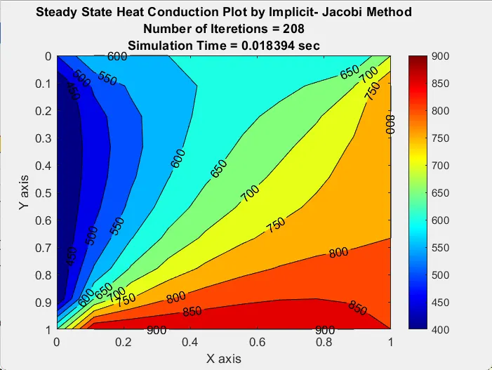
By Jacobi Method
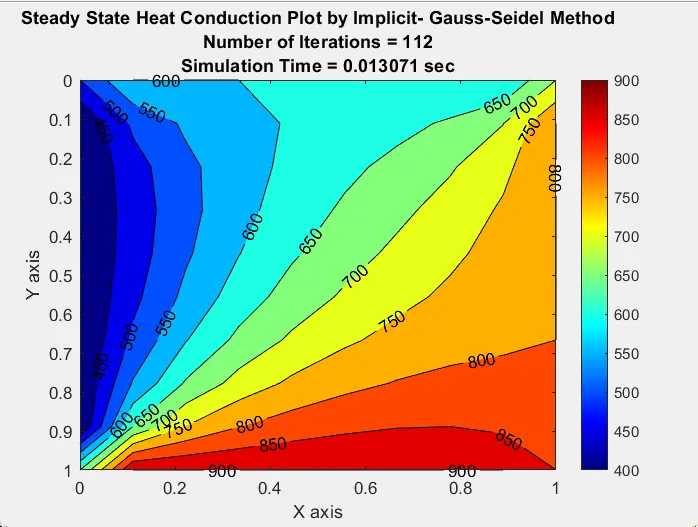
By Gauss-Seidel Method
By Successive Over Relaxation Method
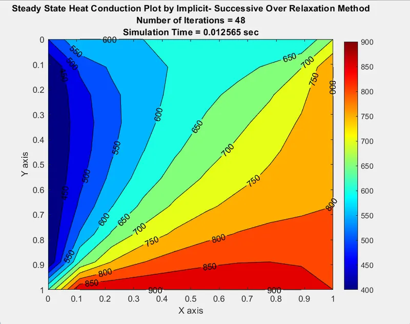
From the above plots, we can see that the Number of Iterations to get converged solution is least for Successive Over Relaxation Method and in increasing order is as follows SOR, Gauss-Seidel and Jacobi Method.
Transient State Implicit Method-
Formulae:
By Jacobi Method
`T_(i,j)^(n+1)=(T_(i,j)^n+k_1*(T_(i-1,j)+T_(i+1,j))^n+k_2*(T_(i,j-1)+T_(i,j+1))^n)/(1+2*k_1+2*k_2)`
By Gauss-Seidel Method
`T_(i,j)^(n+1)=(T_(i,j)^n+k_1*(T_(i-1,j)+T_(i+1,j))^(n+1)+k_2*(T_(i,j-1)+T_(i,j+1))^(n+1))/(1+2*k_1+2*k_2)`
By Successive Over Relaxation Method
`T_(i,j)^(n+1)=(1-omega)*T_(i,j)^n+omega*((T_(i,j)^n+k_1*(T_(i-1,j)+T_(i+1,j))^(n+1)+k_2*(T_(i,j-1)+T_(i,j+1))^(n+1))/(1+2*k_1+2*k_2))`
Main Code:
close all
clear all
clc

% No of Grid Points
nx = 10;
ny = nx;
nt = 1400;

x = linspace(0,1,nx);
y = linspace(0,1,ny);
dx = x(2) - x(1);
dy = y(2) - y(1);

% Error Criteria
tol = 1e-4;

% Boundary conditions
T = 300*ones(nx,ny);
T(:,1) = 400;
T(1,:) = 600;
T(:,ny) = 800;
T(nx,:) = 900;

% Temperature at Corners
T(1,1) = 500;
T(nx,ny) = 850;
T(1,ny) = 700;
T(nx,1) = 650;

T_old = T;
T_initial = T;

% Time step
dt = 0.01;
alpha = 0.3;
k1 = alpha*(dt/dx^2);
k2 = alpha*(dt/dy^2);

% Method Input
method = input('Iterative Method = ');

%% Jacobi Method
if(method==1)
    tic;
    jacobi = 1;
    for p = 1:nt
        error = 9e9;
        while(error>tol)
            for i = 2:(nx-1)
                for j = 2:(ny-1)
                    term1 = 1/(1+(2*k1)+(2*k2));
                    term2 = k1*term1;
                    term3 = k2*term1;
                    H = (T_old(i-1,j))+(T_old(i+1,j));
                    V = (T_old(i,j-1))+(T_old(i,j+1));
                    T(i,j) = (T_initial(i,j)*term1) + (H*term2) + (V*term3);
                end
            end
            error = max(max(abs(T-T_old)));
            T_old = T;
            jacobi = jacobi + 1;
        end
        T_initial = T;
    end
    gauss_seidel_time = toc;

    figure(1)
    contourf(x,y,T,'ShowText','on');
    colormap(jet);
    colorbar;
    set(gca, 'ydir', 'reverse')
    xlabel('X axis')
    ylabel('Y axis')
    text1 = sprintf('Number of Iteretions = %d', jacobi);
    text2 = sprintf('Simulation Time = %f sec', gauss_seidel_time);
    title({'Transeint State Heat Conduction Profile by Implicit- Jacobi Method'; text1; text2});
end

%% Gauss-Seidel Method
if(method==2)
    tic;
    gauss_seidel = 1;
    for p = 1:nt
        error = 9e9;
        while(error>tol)
            for i = 2:(nx-1)
                for j = 2:(ny-1)
                    term1 = 1/(1+(2*k1)+(2*k2));
                    term2 = k1*term1;
                    term3 = k2*term1;
                    H = (T(i-1,j))+(T_old(i+1,j));
                    V = (T(i,j-1))+(T_old(i,j+1));
                    T(i,j) = (T_initial(i,j)*term1) + (H*term2) + (V*term3);
                end
            end
            error = max(max(abs(T-T_old)));
            T_old = T;
            gauss_seidel = gauss_seidel + 1;
        end
        T_initial = T;
    end
    gauss_seidel_time = toc;

    figure(2)
    contourf(x,y,T,'ShowText','on');
    colormap(jet);
    colorbar;
    set(gca, 'ydir', 'reverse')
    xlabel('X axis')
    ylabel('Y axis')
    text1 = sprintf('Number of Iterations = %d', gauss_seidel);
    text2 = sprintf('Simulation Time = %f sec', gauss_seidel_time);
    title({'Transeint State Heat Conduction Profile by Implicit- Gauss-Seidel Method'; text1; text2})
end

%% Successive Over Relaxation Method
if(method==3)
    tic;
    sor=1;
    omega=1.2;
    for p = 1:nt
        error = 9e9;
        while(error>tol)
            for i = 2:(nx-1)
                for j = 2:(ny-1)
                    term1 = (1+(2*k1)+(2*k2))^-1;
                    term2 = k1*term1;
                    term3 = k2*term1;
                    H = T(i-1,j) + T_old(i+1,j);
                    V = T(i,j-1) + T_old(i,j+1);
                    T(i,j) = (T_old(i,j)*(1-omega))+(omega*((T_initial(i,j)*term1)+(H*term2)+(V*term3)));
                end
            end
            error = max(max(abs(T-T_old)));
            T_old = T;
            sor = sor + 1;
        end
        T_initial = T;
    end
    sor_time = toc;

    figure(3)
    contourf(x,y,T,'ShowText','on');
    colormap(jet);
    colorbar;
    set(gca, 'ydir', 'reverse')
    xlabel('X axis')
    ylabel('Y axis')
    text1 = sprintf('Number of Iterations = %d', sor);
    text2 = sprintf('Simulation Time = %f sec', sor_time);
    title({'Transeint State Heat Conduction Profile by Implicit- Successive Over Relaxation Method'; text1; text2});
end
Output:
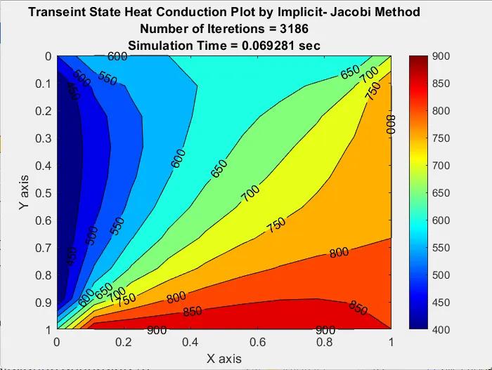
By Jacobi Method
By Gauss-Seidel Method
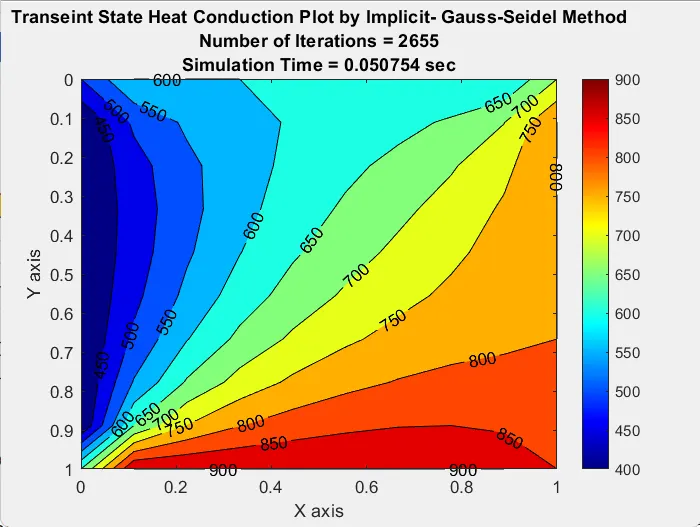
By Successive Over Relaxation Method
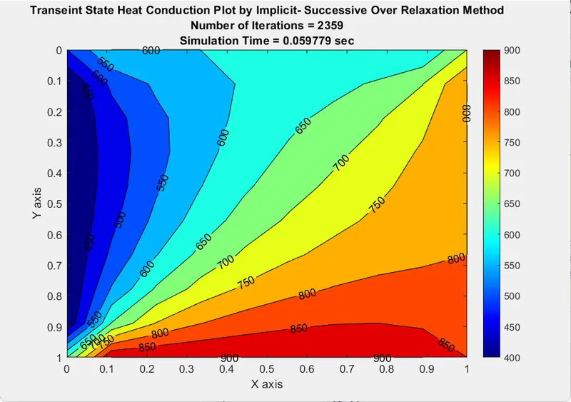
From the above plots, we can see that the Number of Iterations to get converged solution is least for Successive Over Relaxation Method and in increasing order is as follows SOR, Gauss-Seidel and Jacobi Method.
Explicit Transient Method-
Formula:
`T_(i,j)^(n+1)=T_(i,j)^n+k1*(T_(i+1,j)-2*T_(i,j)+T_(i-1,j))^n+k2*(T_(i,j+1)-2*T_(i,j)+T_(i,j-1))^n`
where,
`k_1=(alpha*trianglet)/(trianglex^2) & k_2=(alpha*trianglet)/(triangley^2)`
Main Code:
clear all
close all
clc

nx = 10;
ny = 10;
nt = 300;

x = linspace(0,1,nx);
y = linspace(0,1,ny);
dx = x(2) - x(1);
dy = y(2) - y(1);

T = 300*ones(nx,ny);
T(:,1) = 400;
T(1,:) = 600;
T(:,ny) = 800;
T(nx,:) = 900;

T(1,1) = 500;
T(nx,ny) = 850;
T(1,ny) = 700;
T(nx,1) = 650;

dt = 0.01;
T_old = T;
alpha = 0.3;

k1 = (alpha*dt)/(dx^2);
k2 = (alpha*dt)/(dy^2);

tic;
explicit = 1;
for p = 1:nt
    for i = 2:(nx-1)
        for j = 2:(ny-1)
            term1 = T_old(i-1,j)-2*T_old(i,j)+T_old(i+1,j);
            term2 = T_old(i,j-1)-2*T_old(i,j)+T_old(i,j+1);
            T(i,j) = T_old(i,j)+(k1*term1)+(k2*term2);
        end
    end
    T_old = T;
    explicit = explicit + 1;
end
explicit_time = toc;

figure(1)
contourf(x,y,T,'ShowText','on');
colormap(jet);
colorbar;
set(gca, 'ydir', 'reverse')
xlabel('X-Axis')
ylabel('Y_Axis')
text1 = sprintf('Time = %d sec', dt*nt);
text2 = sprintf('Number of Iteration = %d', explicit);
text3 = sprintf('Simulation Time = %f sec', explicit_time);
title({'Transient State Heat Conduction Profile for Explicit Transient Method'; text1; text2; text3});
Output:
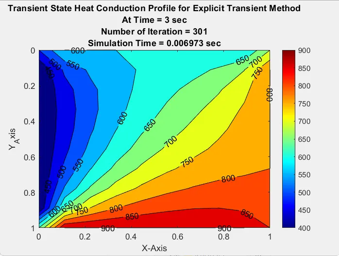
From above plot, we can see that explicit method is converging faster than implicit methods.
Conclusion-
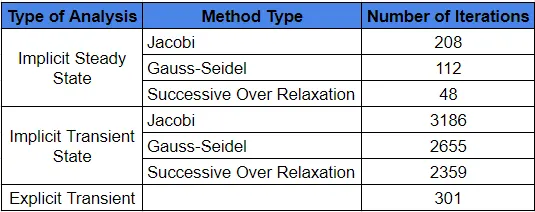
It is evident that,
1. For all analysis methods, the Number of Iterations in increasing order is as follows: Jacobi>Gauss-Seidel>SOR
2. From both Steady State and Transient State Analysis, the number of iterations and simulation time is least for Implicit Steady State Analysis
3. SOR iteration method shows least number of iterations and simulation time in both Steady State and Transient State Analysis