Week 9 - FVM Literature Review
In CFD, there are three methods used for discretizing a PDE:
1. Finite Element Method- In this method, the problem space is divided into discrete elemental areas, usual triangles for 2D applications, and tetrahedra for 3D geometries.
2. Finite Difference Method- Both the spatial domain and time interval (if applicable) are discretized into a finite number of steps and the value o the solution is approximated by solving algebraic equations containing finite differences and values from nearby points.
3. Finite Volume Method- In the finite volume method, volume integrals in a PDE that contain a divergence term are converted to surface integrals, using the divergence theorem. These terms are then evaluated as fluxes at the surfaces of each finite volume. The domain can be discretized in the form of cubic, tetrahedral or polyhedral volumes.
Difference between FDM & FVM-
The finite Difference Method (FDM) has some drawbacks in solving curved boundaries due to the mesh being defined in particular one or two axes which increases the time and extra effort to get the converged results. If one can overcome the boundary condition problem, the method gives very efficient and high-quality results.
On the other hand, the Finite Volume Method (FVM) can be easily used to formulate unstructured meshes. One crucial aspect is the discretization of the fluxes at the boundaries of each control volume. For FVM to be an efficient method, the numerical fluxes are conservative i.e. the quantity of flux entering a control volume is equal to the quantity of flux leaving that control volume and consistent which means the numerical flux of a regular function interpolation tends to the continuous flux as the mesh size tends to zero.
Need for interpolation scheme and flux limiter-
Let's consider the 1D linear heat conduction equation,
`del/(delx) *(alpha(delT)/(delx)) + S = 0`
where 'S' is the source term for heat generation, '`alpha`' is thermal diffusivity and '`(delT)/(delx)`' is temperature gradient.
Solving the above equation using FVM,
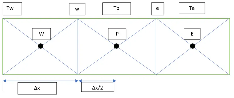
The entire volume is discretized into smaller control volumes as shown in the above image. Let us consider that each volume is formed by the combination of several small volumes dv. So, in order to get that form, a small control volume (dv) as shown below in the figure is multiplied with the governing equation and integrated for the entire volume.
`∫(∂/(∂x) (α (∂T)/(∂x))+s)dv=0`
Rearranging,
`∫(∂/(∂x) (α (∂T)/(∂x)))dv+∫sdv=0`
We know that, dv=A.dx where A is the area
`∫(∂/(∂x) (α ∂T/(∂x)))Adx+∫sdv=0`
`[αA(∂T/∂x)]_w^e+ s ̅dv=0`
The `(delT)/(delx)` term can be found by implementing the Taylor series of 1st order or 2nd order approximations.
`α_e A[(T_e-T_p)/(∆x)]-α_w A[(T_p-T_w)/(∆x)]+ s ̅dv=0`
Since, thermal diffusivity is a function of temperature,
`αA[(T_e-T_p)/(∆x)]-αA[(T_p-T_w)/(∆x)]+ s ̅dv=0`
In case when the thermal diffusivity is not constant, then it should be linearized as follows,
`[Heatflux]_(out)-[Heatflux]_(i n)+Sourceterm=0`
Interpolation schemes are used in evaluating unknown variables at locations other than computational nodes for formulating surface and volume integrals which makes using it necessary in FVM. In the above example, the temperature gradient term can be found or solved with the help of temperatures in the neighboring volumes.
There are different types of interpolation schemes:
1. Upwind interpolation scheme - This interpolation scheme is similar to that of backward or forward finite difference approximation. This scheme approximates the value of some variables at the east face of the control volume.
2. Linear interpolation scheme - This scheme is similar to the central difference scheme. In this scheme, the variables at the center are found by applying the linear interpolation method of values at the two nearest nodes.
3. Quadratic upwind interpolation scheme (QUICK) - This scheme derived the variables by using polynomial fitting. This scheme is third-order accurate and it is prone to oscillations.
4. Hybrid difference scheme - The hybrid difference scheme is the combination of both the central difference scheme and the upwind difference scheme. This scheme is used to find the numerical solution to convection-diffusion problems.
5. Total variation diminishing scheme (TVD) - This scheme is used for solving the hyperbolic partial differential equation in certain discretization schemes. It has a good role in the CFD domain.
Whereas Flux limiters are used in high-resolution schemes to avoid the spurious oscillations that would otherwise occur with high-order spatial discretization schemes due to shocks, discontinuities, or sharp changes in the solution domain. The total variation diminishing (TVD) solution may occur when the flux limiters are applied with a high-resolution scheme to solve the problems. The spatial derivatives can be converted into realistic values by using flux limiters. This is the major concept behind the construction of flux limiter schemes. The flux limiters are used in problems having sharp wave fronts.