Week 11 - Simulation of Flow through a pipe in OpenFoam
Simulation of flow through a pipe in OpenFoam-
Boundary Layer theory:
Consider a fluid entering a circular pipe at uniform velocity, with the no-slip condition. The velocity of the fluid at the mid-section has to increase to keep the mass flow rate through the pipe constant, resulting in a velocity gradient. The hydrodynamic entrance region is the region from the inlet to the point at which the velocity profile becomes fully developed, and its length is the hydrodynamic entrance length.
Hagen-Poiseuille equation:
The Hagen-Poiseuille equation describes the parabolic velocity profile of frictional, laminar pipe flows of incompressible, Newtonian fluids. It states that when a fluid is moving through a pipe velocity will be varying in the radial direction in a particular manner, this is because of the presence of fluid boundary friction, which may be otherwise stated as a no-slip condition.
It is assumed to have no acceleration of flow. Flow resistance offered is shear stress.
Shear stress is `tau=mu*(du)/(dy)`
Hydrodynamic length & Fully Developed flow regions:
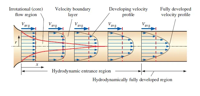
- The figure above shows two regions hydrodynamic entrance region and a fully developed region, the entrance length is the distance a flow travels after entering the pipe.
- This hydrodynamic entrance length refers to the length of the entry region, the area following the pipe entrance where the effect originating from the interior wall of the pipe propagates into the flow as an expanding boundary layer.
- When the boundary layer expands to fill the entire pipe, the developing flow becomes a fully developed flow, where flow characteristics no longer change with increased distance along the pipe.
- The region of flow in which the effects of viscous effects and velocity are sudden changes is called the boundary layer.
- The boundary surface divides the flow in a pipe into two regions, the irrotational flow region, and the boundary layer region
- The viscous affects the velocity changes are significant in the boundary layer region, friction effects are negligible and the velocity essentially remains in the radial direction in the irrotational region
- The thickness of the boundary increases gradually with the flow, when it reaches mid-section the velocity profile becomes fully developed.
- This length where the flow converts to a fully developed region from the entry point is called a hydrodynamic entrance region.
- The flow in this region is called hydrodynamically developed flow since this is the region where the velocity profile develops and keeps changing.
- The flow in the region is fully developed flow and remains constant across the pipe, creating a parabolic velocity profile as shown in the figure above
- The shear stress is directly proportional to the velocity gradient, thus the shear stress at the wall is maximum and the shear stress at the center is minimum.
- The Hydrodynamic entrance length can be calculated using
- `L_e= 0.05*Re*D` where Re is Reynolds number and D is the diameter of the pipe.
Observations based on the Hagen-Poiseuille equation:
- Diameter of pipe `D=0.02m`
- Hydrodynamic entrance length `=0.06∗Re∗D=2.82m`
- Wedge angle `θ=4°`
- Dynamic viscosity of water `μ=0.89e^(−3)Pa-sec`
- The density of water `ρ=997(kg)/m^3`
- Kinematic viscosity `ν=μ/ρ=(0.89e^(−3))/997=8.9268e^(−7)m^2/sec`
- Average velocity `v_(avg)=(μ∗R_e)/(ρ∗D)=0.0937m/sec`
- Velocity profile `u(r)=2*v_(avg)*(1−r^2/R^2)`
- The velocity profile is maximum at the center of the pipe and becomes zero at the pipe wall due to the no-slip condition at the pipe wall.
- `u_max=2⋅v_(avg)*=0.1875m/sec`
- Pressure drop for the fluid in the laminar flow `△p=(32⋅μ⋅v_(avg)⋅L)/D^2=0.0169kPa`
- Shear stress `tau= (2∗μ∗u_max∗r)/R^2`
The sector which is to be created using the blockMeshDict file has a sweep angle of less than 5° since the angle is small the arc can be approximated to a straight line, it can be illustrated as follow,
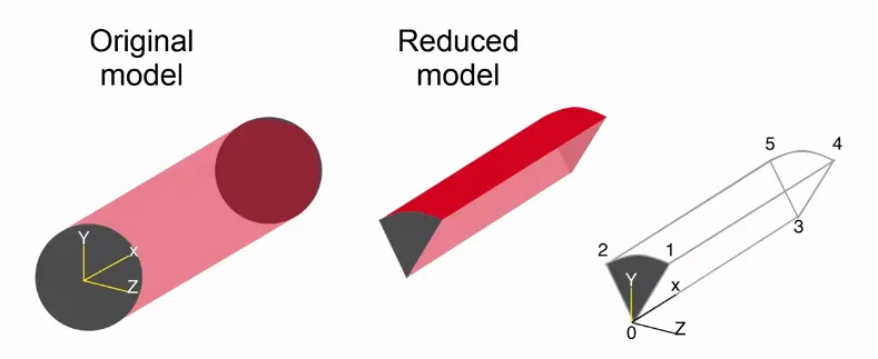
In this simulation angle of 2° is taken accordingly the blockMeshDict file is created by file parsing in Matlab.
Boundaries included are
- inlet, outlet both of which are of type patch
- Front and back which are of type wedge
- No slip wall which is of type wall
- axis which is of type empty
MATLAB code to automate the generation of the blockMeshDict file-
clear all
close all
clc

Re= 2100; % Reynold's Number
D= input('Enter  Diameter of the Pipe ='); % Diameter of the pipe
R=D/2; % Radius of the pipe
theta= input('Enter  Wedge Angle ='); % Wedge Angle
mu=0.89e-3; %Dynamic viscocity @ 25 degree Celsius
rho=997; %Density of water  @ 25 degree Celsius
nu= mu/rho; %Kinematic viscocity  @ 25 degree Celsius

% Analytical Velocity, pressure
L_e= 0.06*Re*D; % Entrance length of the pipe
L_t= L_e + 0.3; % Total length of the pipe
v_avg= (Re*mu)/(rho*D); % Average velocity
v_max= 2*v_avg; % Maximum velocity
Delta_P= (32*mu*v_avg*L_t)/(D^2); % Pressure Drop
kin_P= Delta_P/rho; % Kinematic Pressure

% Finding vertices
v0= [0 0 0];
v1= [0 R*cosd(theta/2) -R*sind(theta/2)];
v2= [0 R*cosd(theta/2) R*sind(theta/2)];
v3= [L_t 0 0];
v4= [L_t R*cosd(theta/2) -R*sind(theta/2)];
v5= [L_t R*cosd(theta/2) R*sind(theta/2)];

%blockMeshDict file.
f1= fopen('blockMeshDict.txt','w'); % create blockmesh file

fprintf(f1,'%s','/*--------------------------------*- C++ -*----------------------------------*');
fprintf(f1,'n');
fprintf(f1,'%s','  =========                 |');
fprintf(f1,'n');
fprintf(f1,'%s','  \      /  F ield         | OpenFOAM: The Open Source CFD Toolbox');
fprintf(f1,'n');
fprintf(f1,'%s','   \    /   O peration     | Website:  https://openfoam.org');
fprintf(f1,'n');
fprintf(f1,'%s','    \  /    A nd           | Version:  9');
fprintf(f1,'n');
fprintf(f1,'%s','     \/     M anipulation  |');
fprintf(f1,'n');
fprintf(f1,'%s','*---------------------------------------------------------------------------*/');
fprintf(f1,'n');
fprintf(f1,'%s','FoamFile');
fprintf(f1,'n');
fprintf(f1,'%s','{');
fprintf(f1,'n');
fprintf(f1,'%s','    version     2.0;');
fprintf(f1,'n');
fprintf(f1,'%s','    format      ascii;');
fprintf(f1,'n');
fprintf(f1,'%s','    class       dictionary;');
fprintf(f1,'n');
fprintf(f1,'%s','    object      blockMeshDict;');
fprintf(f1,'n');
fprintf(f1,'%s','}');
fprintf(f1,'n');
fprintf(f1,'%s','// * * * * * * * * * * * * * * * * * * * * * * * * * * * * * * * * * * * * * //');
fprintf(f1,'n');
fprintf(f1,'n');
fprintf(f1,'%s','convertToMeters 1;');
fprintf(f1,'n');
fprintf(f1,'n');

    b1=blanks(5);
    b2=blanks(6);
    b3=blanks(7);
    b4=blanks(4);

% vertices
fprintf(f1,'vertices n');
fprintf(f1,'(n');
fprintf(f1,b4,'%s n','(');
v_0=fprintf(f1,'(%f %f %f) n',v0(1),v0(2),v0(3));
fprintf(f1,b4,'%s','(');
v_1=fprintf(f1,'(%f %f %f)n',v1(1),v1(2),v1(3));
fprintf(f1,b4,'%s','(');
v_2=fprintf(f1,'(%f %f %f)n',v2(1),v2(2),v2(3));
fprintf(f1,b4,'%s','(');
v_3=fprintf(f1,'(%f %f %f)n',v3(1),v3(2),v3(3));
fprintf(f1,b4,'%s','(');
v_4=fprintf(f1,'(%f %f %f)n',v4(1),v4(2),v4(3));
fprintf(f1,b4,'%s','(');
v_5=fprintf(f1,'(%f %f %f)n',v5(1),v5(2),v5(3));
fprintf(f1,'n);n');

%  blocks creation
fprintf(f1,'nblocksn');
fprintf(f1,'(n');
fprintf(f1,b4,'%s','(');
fprintf(f1,'%s','hex (0 1 2 0 3 4 5 3)');

%  mesh generation
m1= input('Enter no. of mesh element along X-axis:');
m2= input('Enter no. of mesh element along Y-axis:');
m3= input('Enter no. of mesh element along Z-axis:');

fprintf(f1,blanks(1),'%s','(');
fprintf(f1,'(%2.0f %1.0f %3.0f)',m1,m2,m3);
fprintf(f1,'%s',' simpleGrading (1 1 1)');
fprintf(f1,'n);');

%  edges creation
fprintf(f1,'nedgesn');
fprintf(f1,'(n');
fprintf(f1,'%s   arc 1 2 (0 %f 0)',blanks(1),R);
fprintf(f1,'n%s   arc 4 5 (%f %f 0)',blanks(1),L_t,R);
fprintf(f1,'n);nn');

% boundary conditions
% axis
fprintf(f1,'boundaryn(n');
fprintf(f1,'%s','   axis');
fprintf(f1,'n   {n');
fprintf(f1,'%s',blanks(10),'type empty;');
fprintf(f1,'n');
fprintf(f1,'%s',blanks(10),'faces');
fprintf(f1,'n');
fprintf(f1,'%s',blanks(10),'(');
fprintf(f1,'n');
fprintf(f1,'%s',blanks(13),'(0 3 3 0)');
fprintf(f1,'n');
fprintf(f1,'%s',blanks(10),');');
fprintf(f1,'n   }n');

% fixedwalls
fprintf(f1,'%s','   fixedWalls');
fprintf(f1,'n   {n');
fprintf(f1,'%s',blanks(10),'type wall;');
fprintf(f1,'n');
fprintf(f1,'%s',blanks(10),'faces');
fprintf(f1,'n');
fprintf(f1,'%s',blanks(10),'(');
fprintf(f1,'n');
fprintf(f1,'%s',blanks(13),'(2 1 4 5)');
fprintf(f1,'n');
fprintf(f1,'%s',blanks(10),');');
fprintf(f1,'n   }n');

% front
fprintf(f1,'%s','   front');
fprintf(f1,'n   {n');
fprintf(f1,'%s',blanks(10),'type symmetry;');
fprintf(f1,'n');
fprintf(f1,'%s',blanks(10),'faces');
fprintf(f1,'n');
fprintf(f1,'%s',blanks(10),'(');
fprintf(f1,'n');
fprintf(f1,'%s',blanks(13),'(1 0 3 4)');
fprintf(f1,'n');
fprintf(f1,'%s',blanks(10),');');
fprintf(f1,'n   }n');

% back
fprintf(f1,'%s','   back');
fprintf(f1,'n   {n');
fprintf(f1,'%s',blanks(10),'type symmetry;');
fprintf(f1,'n');
fprintf(f1,'%s',blanks(10),'faces');
fprintf(f1,'n');
fprintf(f1,'%s',blanks(10),'(');
fprintf(f1,'n');
fprintf(f1,'%s',blanks(13),'(2 5 3 0)');
fprintf(f1,'n');
fprintf(f1,'%s',blanks(10),');');
fprintf(f1,'n   }n');

% inlet
fprintf(f1,'%s','   inlet');
fprintf(f1,'n   {n');
fprintf(f1,'%s',blanks(10),'type patch;');
fprintf(f1,'n');
fprintf(f1,'%s',blanks(10),'faces');
fprintf(f1,'n');
fprintf(f1,'%s',blanks(10),'(');
fprintf(f1,'n');
fprintf(f1,'%s',blanks(13),'(0 1 2 0)');
fprintf(f1,'n');
fprintf(f1,'%s',blanks(10),');');
fprintf(f1,'n   }nn');

% outlet
fprintf(f1,'%s','   outlet');
fprintf(f1,'n   {n');
fprintf(f1,'%s',blanks(10),'type patch;');
fprintf(f1,'n');
fprintf(f1,'%s',blanks(10),'faces');
fprintf(f1,'n');
fprintf(f1,'%s',blanks(10),'(');
fprintf(f1,'n');
fprintf(f1,'%s',blanks(13),'(3 5 4 3)');
fprintf(f1,'n');
fprintf(f1,'%s',blanks(10),');');
fprintf(f1,'n   }nn');

fprintf(f1,'n);n');

fprintf(f1,'nmergePatchPairs');
fprintf(f1,'n(n);nn');

fprintf(f1,'%s','// * * * * * * * * * * * * * * * * * * * * * * * * * * * * * * * * * * * * * //');
fclose(f1);

% shear stress
r = linspace(0, 0.01, 100);
for i = 1:length(r)
    tau(i) = (2*mu*v_max*abs(r(i)))/R^2;
end
plot(r, tau, 'linewidth', 2)
grid on
xlabel('Along Radius of the Pipe')
ylabel('Shear Stress')
legend('Shear Stress (calculated)')
The water flows through the pipe of 20 mm diameter at a velocity of 0.0935m/s of Reynold's number less than 2100, hence the laminar flow is considered for the project.
When the above Matlab codes are run we get a text file 'output.txt' as output, which is nothing but the blockMeshDict file, this file is copied inside the system directory of the icoFoam case setup.
In order to start with the simulation, we will need to open the Ubuntu terminal and search for the OpenFOAM tutorial directory by giving input of 'tut'. For this challenge, we will be using the 'icoFoam' solver with the 'cavity' section which can be found in the 'incompressible' tutorial folder. In order to not make changes in OpenFOAM official tutorials, we then copy the 'cavity' folder and paste it into the OpenFOAM run folder using the command 'cp -r cavity $FOAM_RUN/flowthroughpipe'.
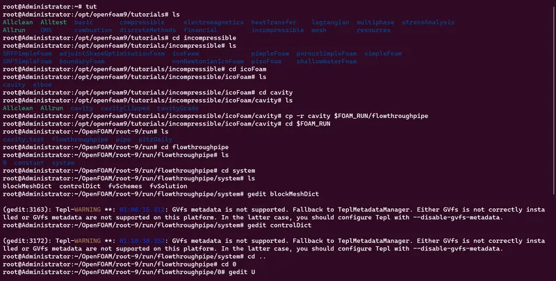
There are four script files in the 'system' folders and by opening them, we can create a domain and provide the required specifications by using the command 'gedit'.
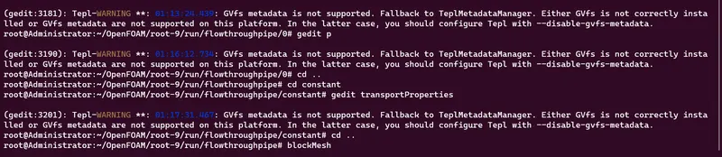
BlockMeshDict file generated from the above code is as shown below:
/*--------------------------------*- C++ -*----------------------------------*
  =========                 |
  \      /  F ield         | OpenFOAM: The Open Source CFD Toolbox
   \    /   O peration     | Website:  https://openfoam.org
    \  /    A nd           | Version:  9
     \/     M anipulation  |
*---------------------------------------------------------------------------*/
FoamFile
{
    version     2.0;
    format      ascii;
    class       dictionary;
    object      blockMeshDict;
}
// * * * * * * * * * * * * * * * * * * * * * * * * * * * * * * * * * * * * * //

convertToMeters 1;

vertices
(
    (0.000000 0.000000 0.000000)
    (0.000000 0.009994 -0.000349)
    (0.000000 0.009994 0.000349)
    (2.820000 0.000000 0.000000)
    (2.820000 0.009994 -0.000349)
    (2.820000 0.009994 0.000349)

);

blocks
(
    hex (0 3 4 1 0 3 5 2) (200 20 1) simpleGrading (1 0.1 1)
);
edges
(
    arc 1 2 (0 0.010000 0)
    arc 4 5 (2.820000 0.010000 0)
);

boundary
(
   axis
   {
          type empty;
          faces
          (
             (0 3 3 0)
          );
   }
   fixedWalls
   {
          type wall;
          faces
          (
             (2 1 4 5)
          );
   }
   front
   {
          type wedge;
          faces
          (
             (1 0 3 4)
          );
   }
   back
   {
          type wedge;
          faces
          (
             (2 5 3 0)
          );
   }
   inlet
   {
          type patch;
          faces
          (
             (0 1 2 0)
          );
   }

   outlet
   {
          type patch;
          faces
          (
             (3 5 4 3)
          );
   }


);

mergePatchPairs
(
);

// * * * * * * * * * * * * * * * * * * * * * * * * * * * * * * * * * * * * * //
controlDict file:
Since the inlet velocity of water is 0.09 m/s, the same is provided in the U file as shown above.
The total time until which the simulations are to be run is calculated,
`v=l/t`
`v=0.09m/s`
`l=2.82m`
Therefore, t = 2.82/0.09 = 31.33sec, which implies at a velocity of 0.09m/s fluid takes 31.33sec to complete one pass.
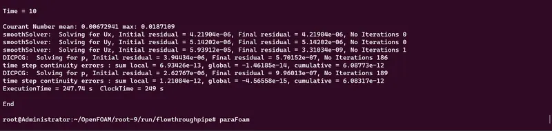
So total time of 10sec is provided in the controlDict file, the time step is determined using the trial and error method. In this case time, step delta t = 0.005 sec is used under which the courant number is well under the max value of C = 1.
/*--------------------------------*- C++ -*----------------------------------*
  =========                 |
  \      /  F ield         | OpenFOAM: The Open Source CFD Toolbox
   \    /   O peration     | Website:  https://openfoam.org
    \  /    A nd           | Version:  9
     \/     M anipulation  |
*---------------------------------------------------------------------------*/
FoamFile
{
    format      ascii;
    class       dictionary;
    location    "system";
    object      controlDict;
}
// * * * * * * * * * * * * * * * * * * * * * * * * * * * * * * * * * * * * * //

application     icoFoam;

startFrom       startTime;

startTime       0;

stopAt          endTime;

endTime         10;

deltaT          0.005;

writeControl    timeStep;

writeInterval   20;

purgeWrite      0;

writeFormat     ascii;

writePrecision  6;

writeCompression off;

timeFormat      general;

timePrecision   6;

runTimeModifiable true;


// ************************************************************************* //
Velocity file:
/*--------------------------------*- C++ -*----------------------------------*
  =========                 |
  \      /  F ield         | OpenFOAM: The Open Source CFD Toolbox
   \    /   O peration     | Website:  https://openfoam.org
    \  /    A nd           | Version:  9
     \/     M anipulation  |
*---------------------------------------------------------------------------*/
FoamFile
{
    format      ascii;
    class       volVectorField;
    object      U;
}
// * * * * * * * * * * * * * * * * * * * * * * * * * * * * * * * * * * * * * //

dimensions      [0 1 -1 0 0 0 0];

internalField   uniform (0.0936 0 0);

boundaryField
{
    inlet
    {
        type            fixedValue;
        value           uniform (0.0936 0 0);
    }

    outlet
    {
        type            zeroGradient;
    }

    fixedWalls
    {
        type            noSlip;
    }

    front
    {
        type            wedge;
    }

    back
    {
        type            wedge;
    }

    axis
    {
        type            empty;
    }
}

// ************************************************************************* //
Pressure file:
/*--------------------------------*- C++ -*----------------------------------*
  =========                 |
  \      /  F ield         | OpenFOAM: The Open Source CFD Toolbox
   \    /   O peration     | Website:  https://openfoam.org
    \  /    A nd           | Version:  9
     \/     M anipulation  |
*---------------------------------------------------------------------------*/
FoamFile
{
    format      ascii;
    class       volScalarField;
    object      p;
}
// * * * * * * * * * * * * * * * * * * * * * * * * * * * * * * * * * * * * * //

dimensions      [0 2 -2 0 0 0 0];

internalField   uniform 0;

boundaryField
{
    inlet
    {
        type            zeroGradient;
    }

    outlet
    {
        type            fixedValue;
        value           uniform 0;
    }

    fixedWalls
    {
        type            zeroGradient;
    }

    front
    {
        type            wedge;
    }

    back
    {
        type            wedge;
    }

    axis
    {
        type            empty;
    }
}

// ************************************************************************* //
transportProperties file:
/*--------------------------------*- C++ -*----------------------------------*
  =========                 |
  \      /  F ield         | OpenFOAM: The Open Source CFD Toolbox
   \    /   O peration     | Website:  https://openfoam.org
    \  /    A nd           | Version:  9
     \/     M anipulation  |
*---------------------------------------------------------------------------*/
FoamFile
{
    format      ascii;
    class       dictionary;
    location    "constant";
    object      transportProperties;
}
// * * * * * * * * * * * * * * * * * * * * * * * * * * * * * * * * * * * * * //

nu              [0 2 -1 0 0 0 0] 8.9268e-07;


// ************************************************************************* //
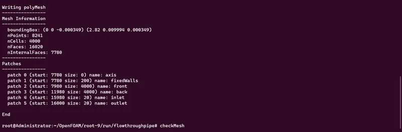
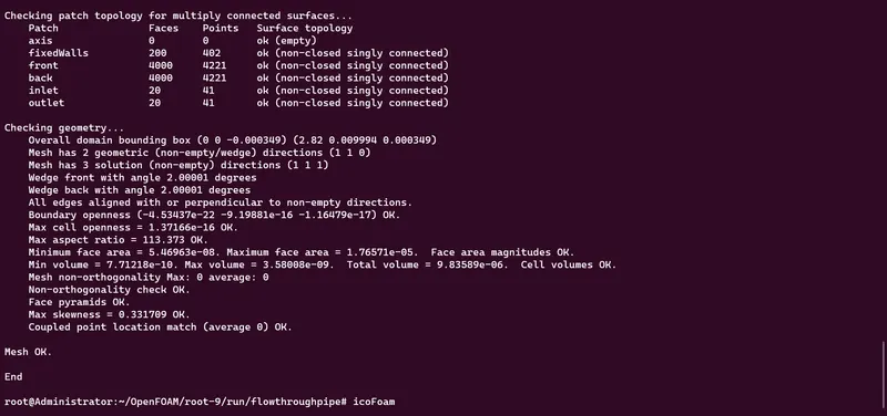
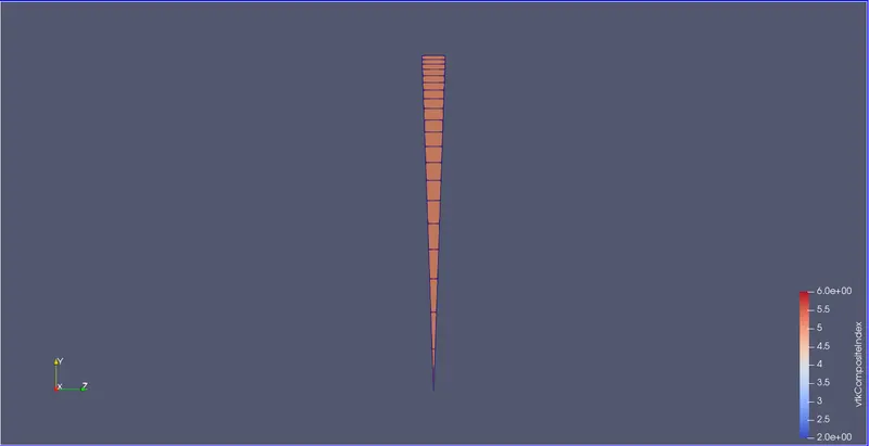
Now, as our problem statement is set we will have to run 'blockMesh' and 'checkMesh' commands. And to check our mesh we have to use the command 'paraFoam' to plot the mesh. To solve the problem statement we have to use the command 'icoFoam'.
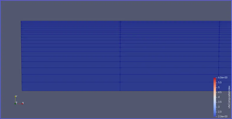
Mesh Grid-
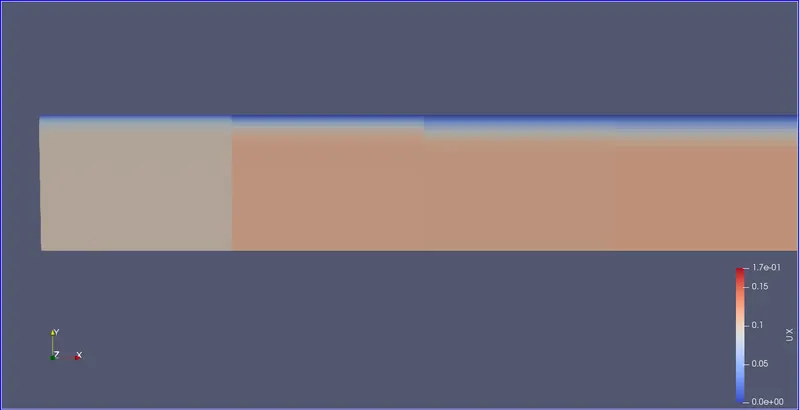
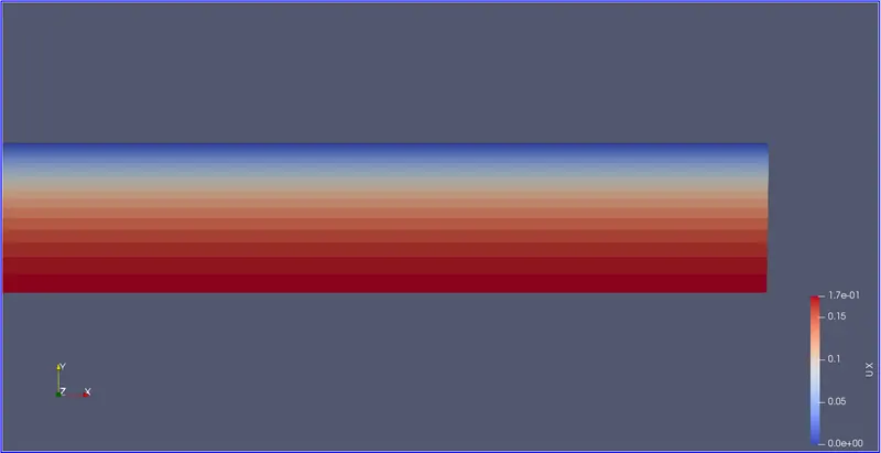
Velocity contour-
Inlet:
Outlet:
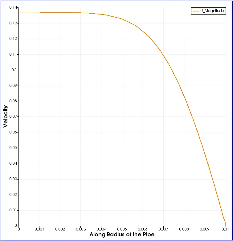
Velocity Plots-
At x=0.25m
At x=0.5m
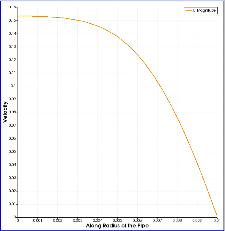
At x=0.75m
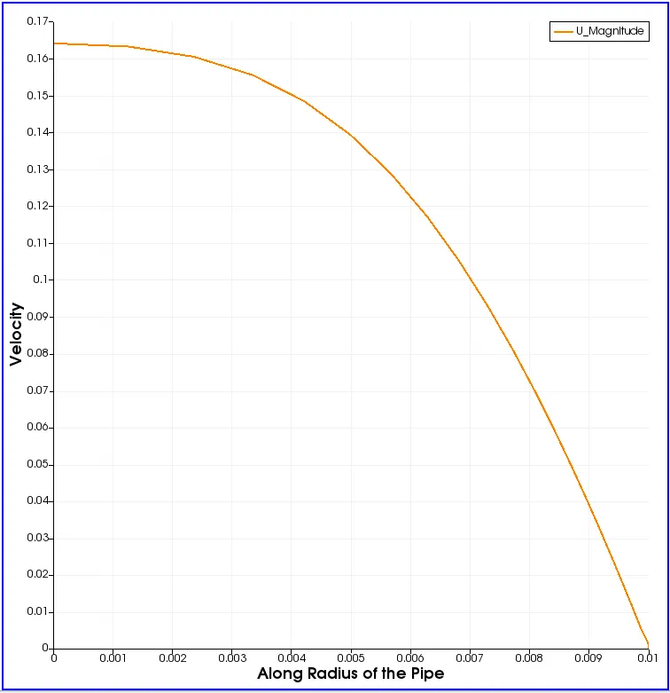
At x=1m
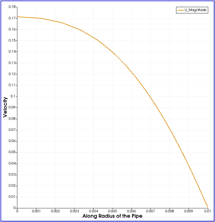
At x=1.5m
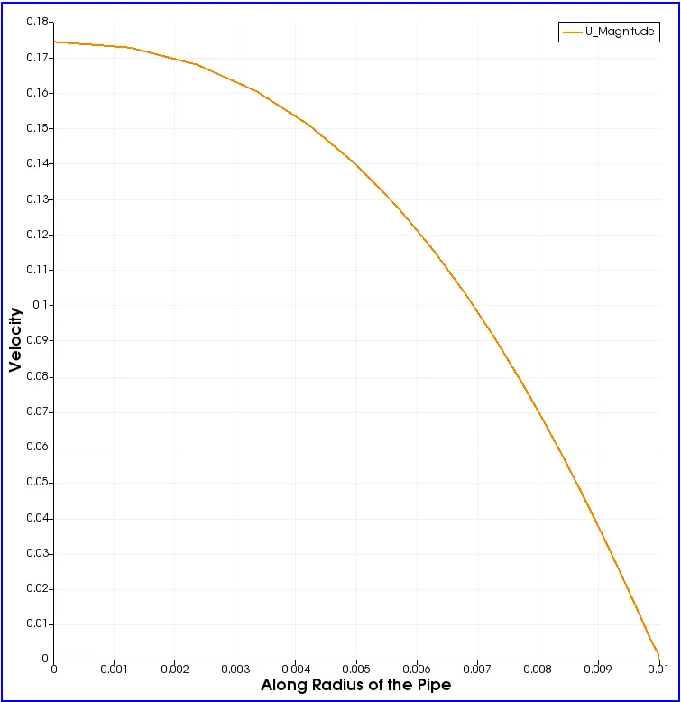
At x=2m
At x=2.52m
At x=2.82m
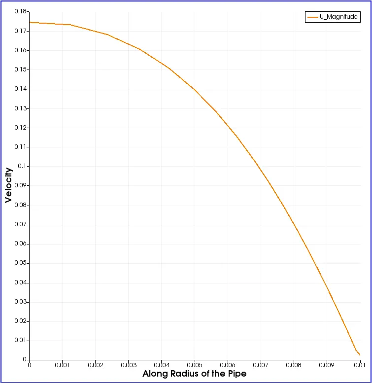
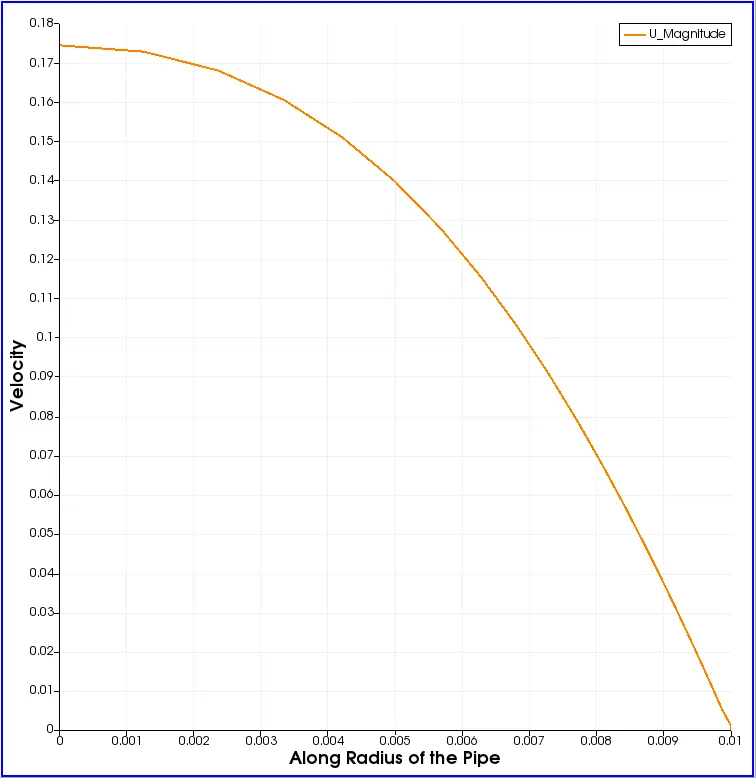
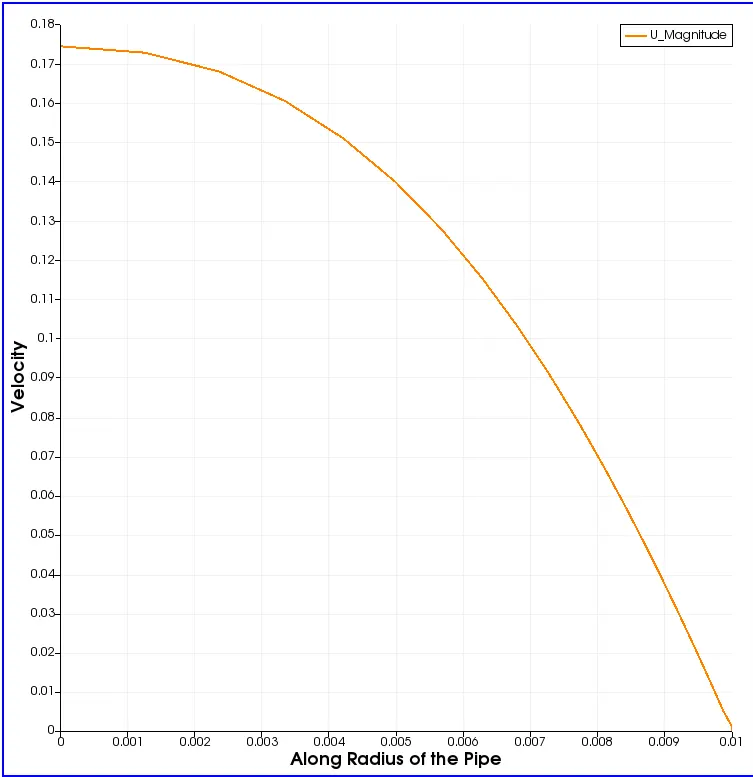
We can see that after 2.52m the velocity profile remains unchanged which implies that the flow is fully developed. By calculation, the Hydro dynamic length is obtained to be 2.52m, where the velocity profile is fully developed. The maximum velocity obtained by OpenFoam is 0.174m/sec.
It is observed that the velocity profile gradually increased from the inlet to the outlet. The velocity profile is observed to increase slowly at different lengths of pipe and also it reached maximum velocity at the outlet. This region is called a fully developed region as the velocity profile completely develops at the outlet.
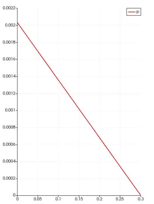
At the walls, the velocity remains zero as we considered no-slip boundary conditions. As the flow progress gradually, the boundary layers develop and the adjacent layers tend to slow down. Because of this, the velocity at the center increases. Hence, because of the pressure difference obtained from the equations, the velocity profile obeys Hagen Poiseuille's equation. Hence velocity profile matches Hagen Poiseuille's equation.
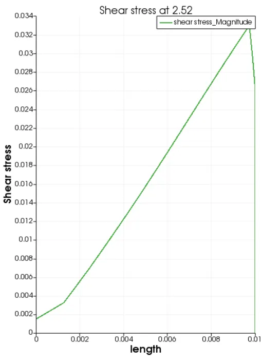
Shear stress-
When the fluid is moving, shear stresses are developed as the particles in the flow move relative to each other. For a fluid flowing in a pipe, the fluid velocity remains zero at the pipe wall. Shear force is generated because of the adjacent layer of the fluid that moves at different velocities.
Shear stress can be calculated as under `tau=mu**frac{du}{dr}`
where
`tau=`Shear stress in Pascal
`mu=`Dynamic viscosity of water in Pascal-sec
`(du)/(dr)=`Velocity gradient
Shear stress plot obtained in OpenFoam:
Shear stress plot obtained in Matlab:
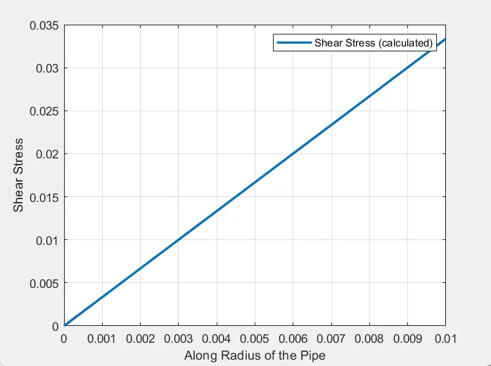
Conclusion-
- Hydro dynamic length is obtained to be 2.52m, where the velocity profile is fully developed.
- The velocity profile gradually increases from inlet to outlet. It remains constant after the flow is fully developed.
- Analytical velocity profile and velocity obtained in OpenFOAM match very well, where velocity is maximum at the center and parabolically decreases toward the wall.
- Shear stress is zero at the center of the pipe and increases linearly toward the wall, the graph obtained from OpenFOAM is close to an analytical result.
- The irregularities can be observed in the shear stress profile because of the "finite volume method". At nodes intersection the value of shear stress increases, this can be reduced by increasing the number of grid points which in turn will increase the computational time.
- Maximum velocity and pressure drop value are obtained for fully developed flow.
- The simulation is done for a wedge angle of 4 degrees but the values will be the same when the simulation is performed for the wedge angle 2degree and 3degree since the flow is steady and incompressible.