Week 1- Mixing Tee

Mixing Tee

Aim:To set up steady-state simulations to compare the mixing effectiveness when hot inlet temperature is 36⁰C & the cold inlet is at 19⁰C.

Objectives:

1.To set up steady-state simulations (Using the k-epsilon and k-omega SST model)

Case 1

• Short mixing tee with a hot inlet velocity of 3m/s.
• Momentum ratio of 2, 4

Case 2

• Long mixing tee with a hot inlet velocity of 3m/s.
• Momentum ratio of 2, 4.

2.To compare the following values from the 2 cases. (in a table)

1. Cell count
2. Average outlet temperature
3. Number of iterations for convergence

Introduction:In this study we have created two versions of the mixing tee. One of them is longer than the other.We are going to find effectiveness of mixing tee.The function of mixing Tee is to provide proper mixing of quantities to get the desired result at the outlet.By controlling the velocity of chilled air we can get the desired temperature in the room.

Theory:Mixing tee is a device which uses specifically engineered internal geometry to mix two fluid streams into one steam, efficiently. Hot air and cold air are going to be mixed in mixing tee. They will have different velocities. We will use two different mixing tee distinguished with length and analyse the effect of length on mixing.

Momentum ratio = velocity at cold inlet / velocity at hot inlet

Procedure:

Case 1:

• Short mixing tee with a hot inlet velocity of 3m/s.(k-omega SST model)
• Momentum ratio of 2

1. Open new project, by clicking on Fluid flow (Fluent) in Ansys workbench.

2. Set gemotry to import mixing tee model. It will redirect to Spaceclaim, Ansys’s geometry model manipulator.

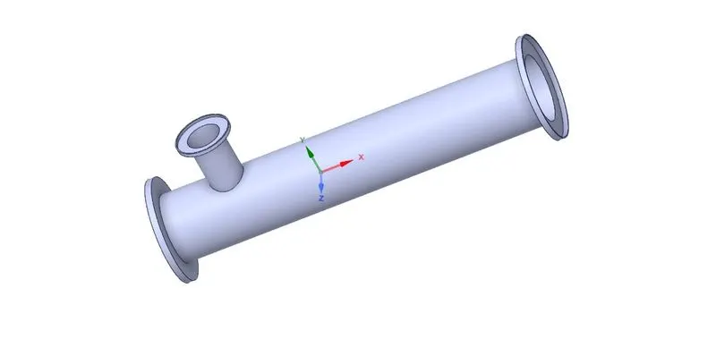
• Extract the volume of fluid flow and suppress the solidmodel.

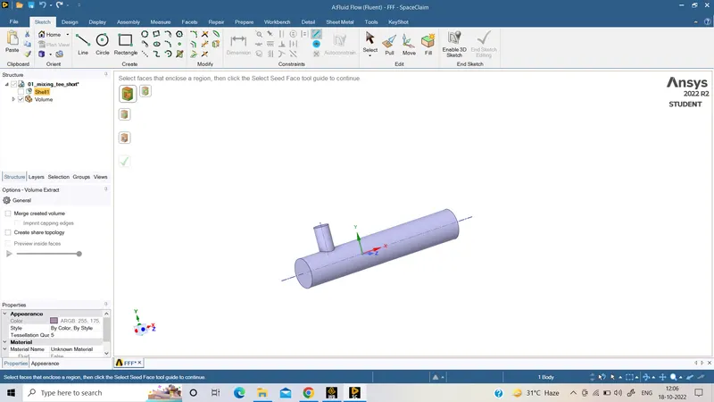
• Exit from spaceclaim and open the mesh.

3.Creat the mesh:

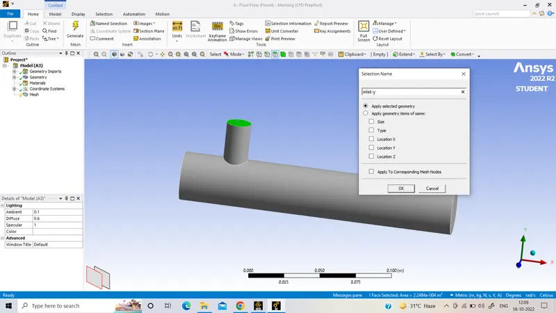
• To set the boundary name we have to click cntrl +F (to select the face ) and N to add selection name i.e.

inlet -y,inlet-x,outlet,walls.

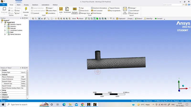
• Generation of the mesh by right clicking the mesh and selecting generate mesh.

Checking the quality of mesh :

• change in the quality :mesh metric:element metric

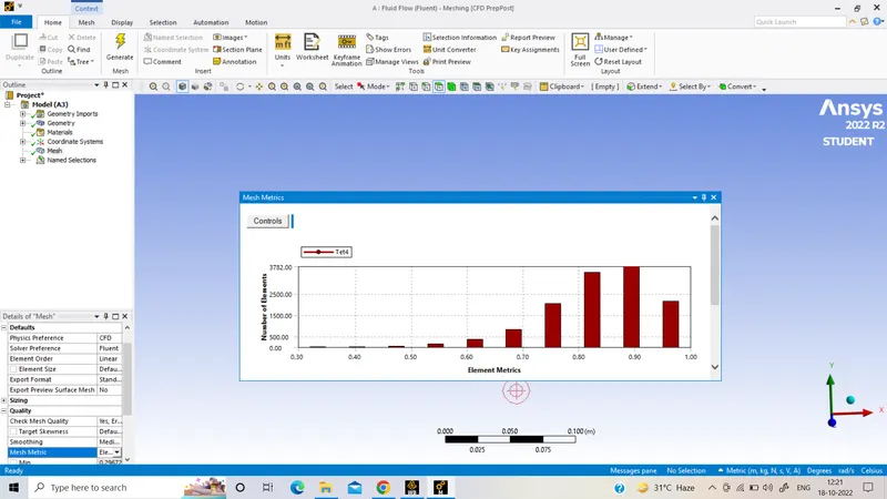
• Close the mesh and update the mesh.

4. Make the setup:

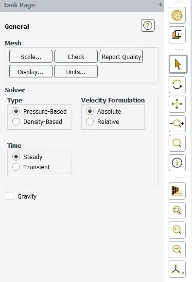
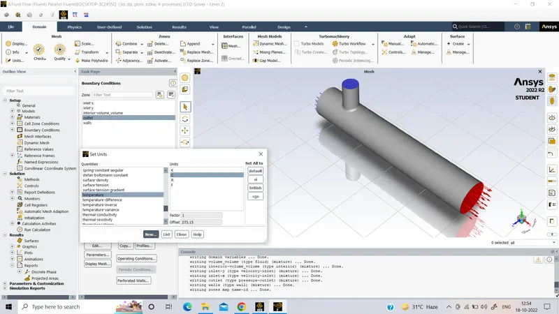
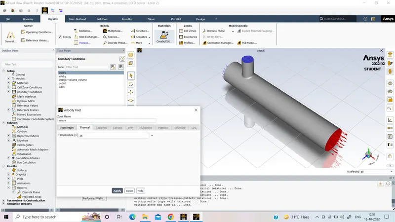
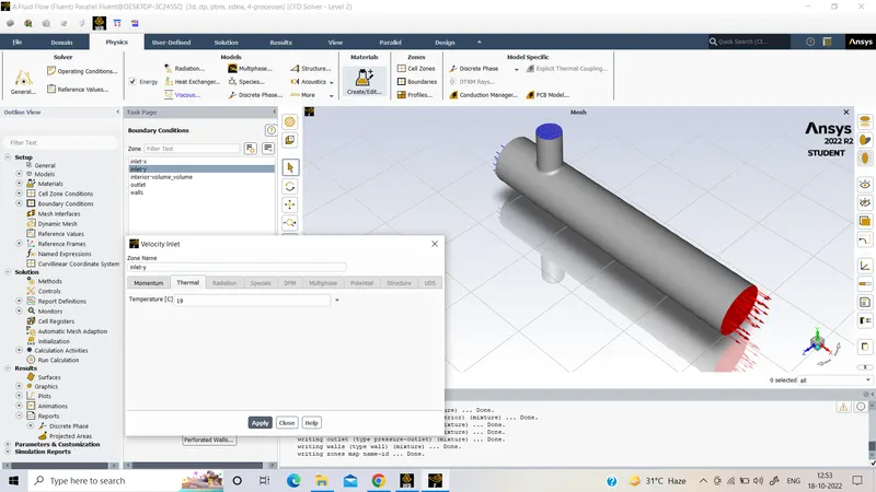
• set the temperature in degree celcious

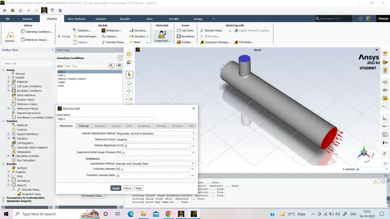
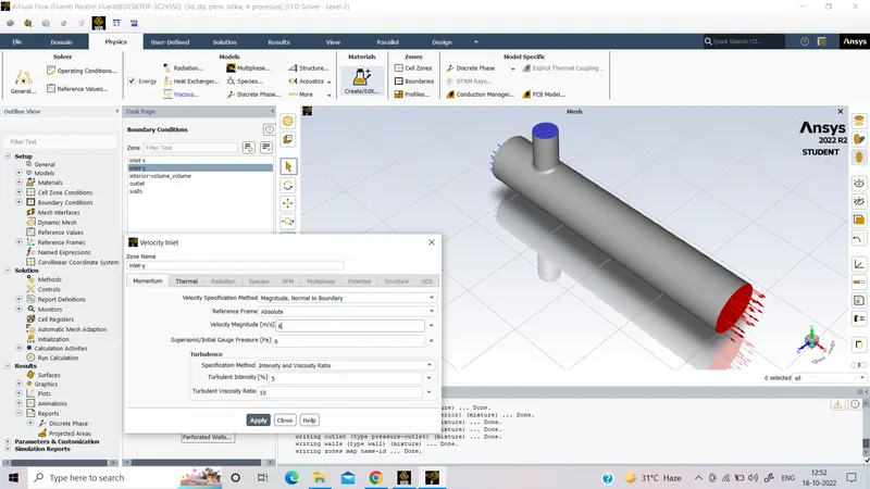
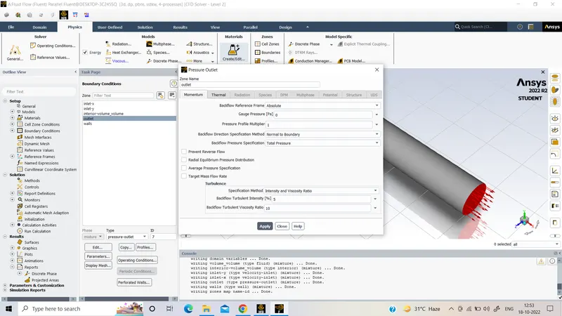
• set boundary conditions

Solution:

• set the physics
• add definations
• intialize the solution
• run calculation by providing suitable no of iterations

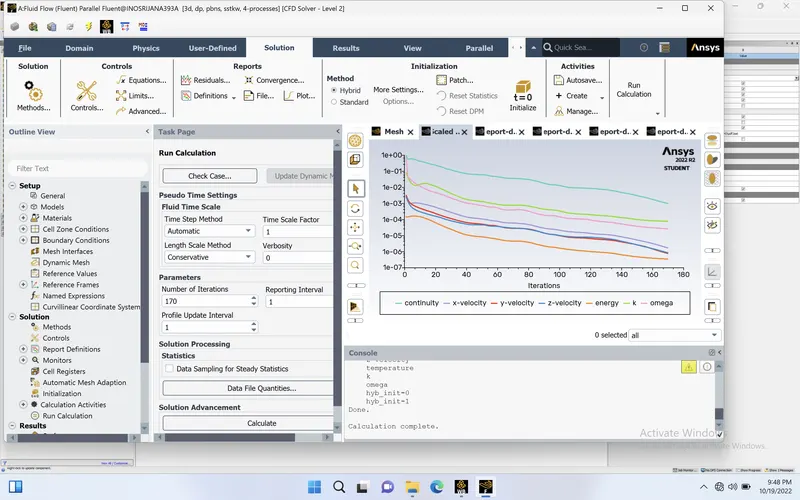
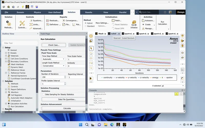
Residuals of governing and transport equations :

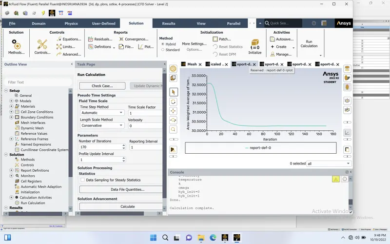
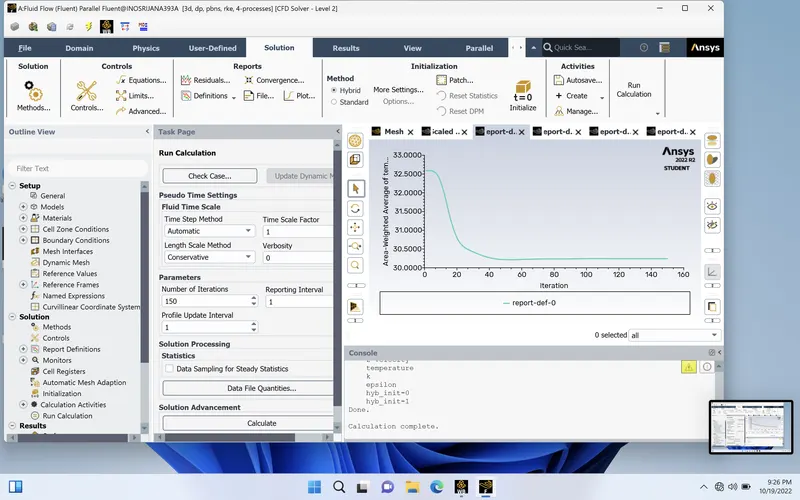
Area weighted avg of temerature at the outlet:

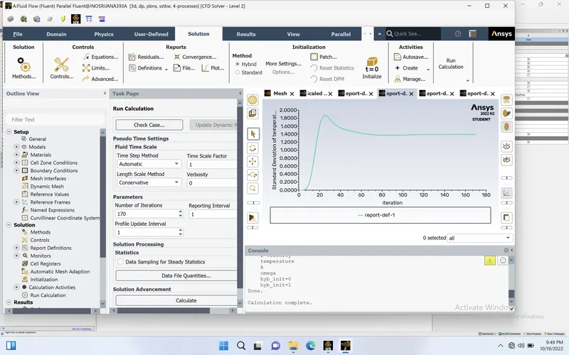
Standard daviation of temperature at the outlet:

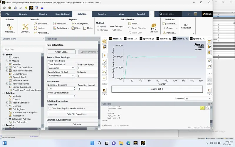
Area weighted avg of velocity at the outlet:

5.Result analysis:

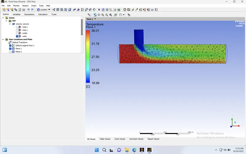
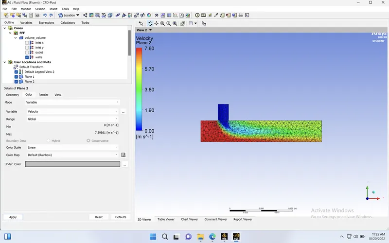
Velocity and temperature contour plots on the cut planes along and across the pipe

Temperature Distribution: plane 1

Velocity Distribution:plane 1

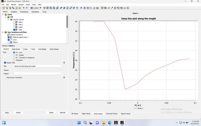
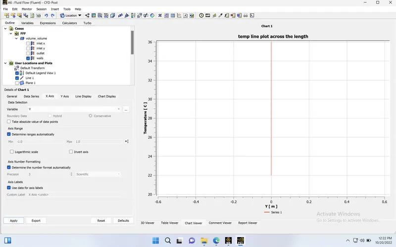
Velocity and temperature line plots along and across the length of the pipe:

Temperature line plots along the length of the pipe:

Temp line plots across the length of the pipe:

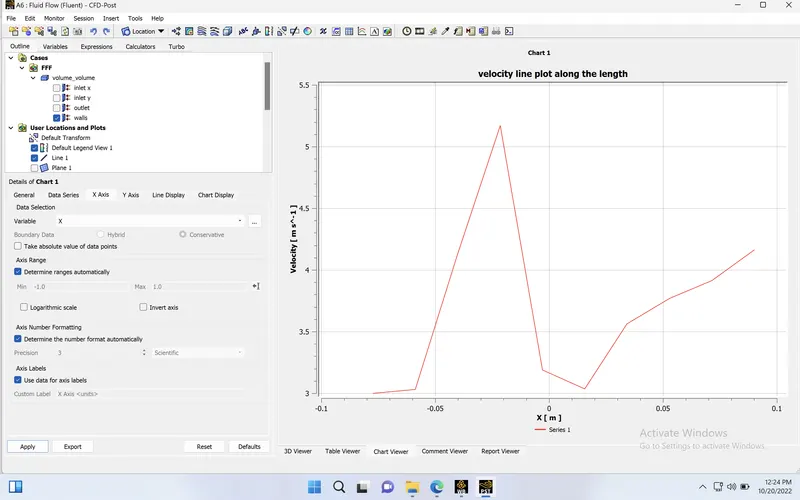
Velocity line plots along the length of the pipe:

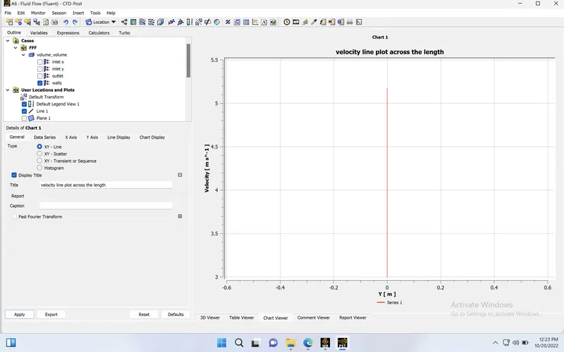
Velocity line plots across the length of the pipe:

Short mixing tee with a hot inlet velocity of 3m/s : k-epsilon model: Momentum ratio of 2

solution:

Residuals of governing and transport equations :

Area weighted avg of temerature at the outlet:

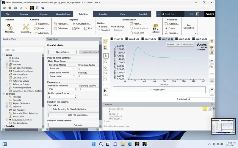
Standard deviation of temerature at the outlet:

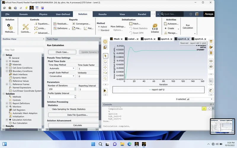
Area weighted avg of velocity at the outlet:

Result analysis:

Velocity and temperature contour plots on the cut planes along and across the pipe

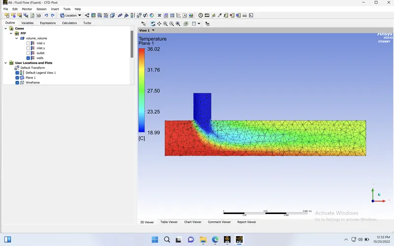
Temperature Distribution:plane1

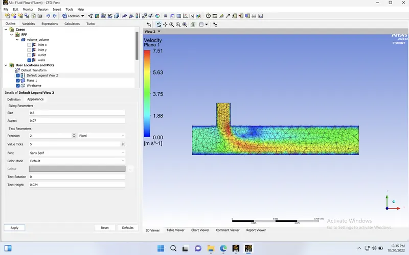
Velocity Distribution:plane1

Velocity and temperature line plots along and across the length of the pipe:

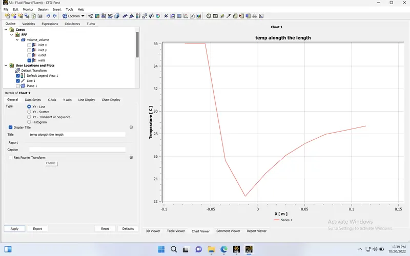
Temperature line plots along length of the pipe:

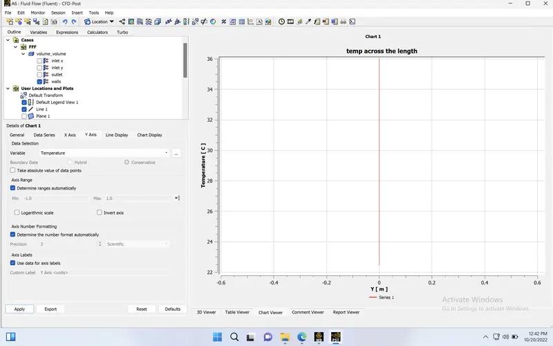
Temperature line plots across length of the pipe:

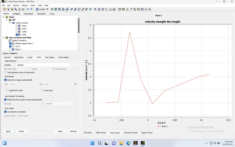
Velocity line plots along length of the pipe:

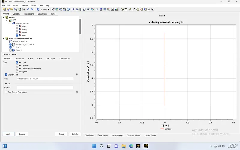
Velocity line plots across length of the pipe:

Short mixing tee with a hot inlet velocity of 3m/s :k-epsilon model: Momentum ratio of 4

Solution:

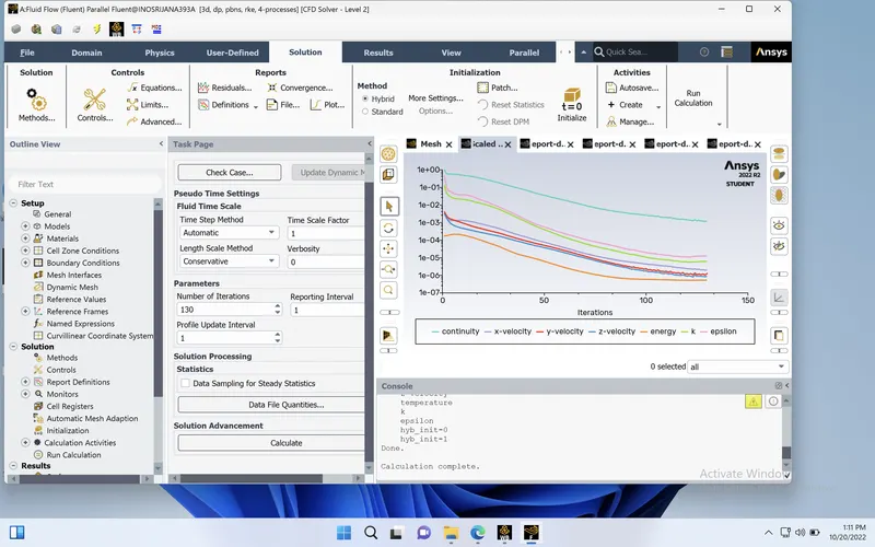
Residuals of governing and transport equations :

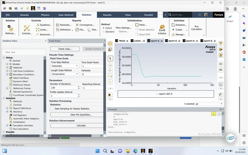
Area weighted avg of temp at the outlet:

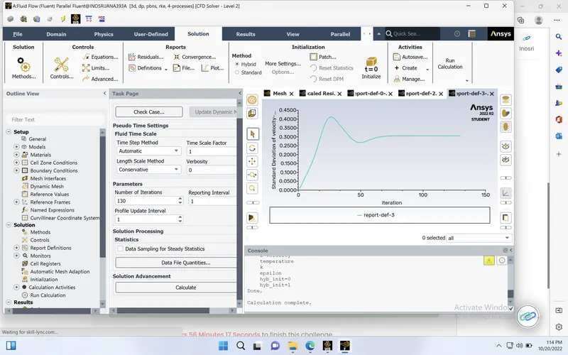
Standard deviation of temp at the outlet:

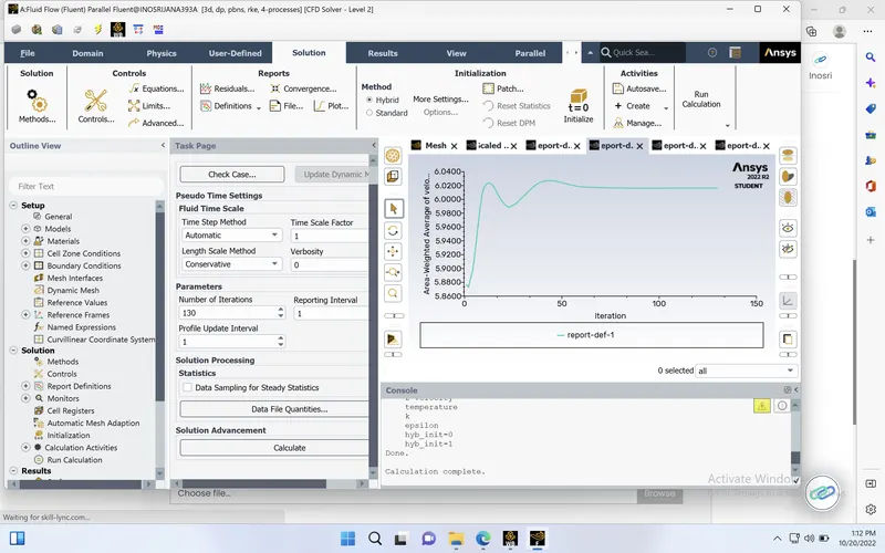
Area weighted avg of velocity at the outlet:

Result analysis:

Velocity and temperature contour plots on the cut planes along and across the pipe

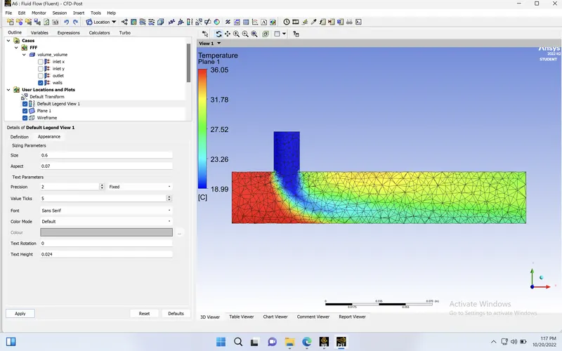
Temperature Distribution:plane 1

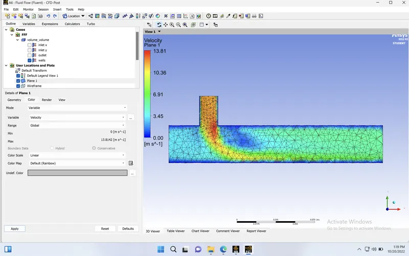
Velocity Distribution:plane1

Velocity and temperature line plots along and across the length of the pipe:

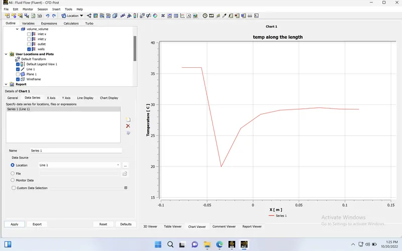
Temperature line plots along length of the pipe:

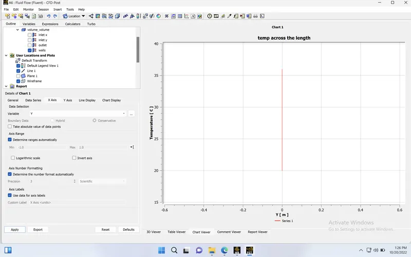
Temperature line plots across length of the pipe:

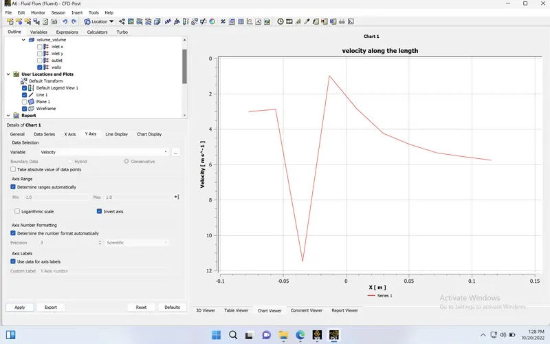
Velocity line plots along length of the pipe:

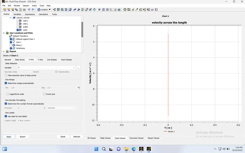
Velocity line plots across length of the pipe:

Long mixing tee with a hot inlet velocity of 3m/s : k-epsilon model: Momentum ratio of 2

solution:

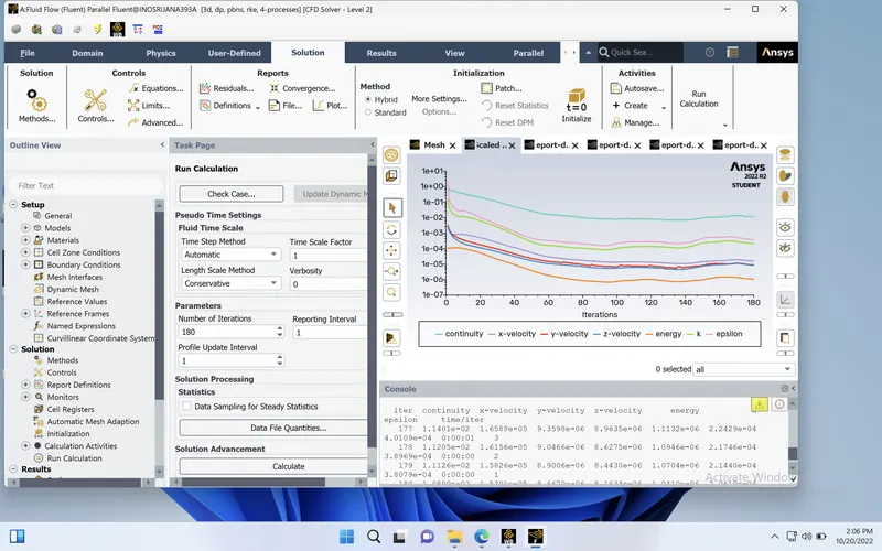
Residuals of governing and transport equations :

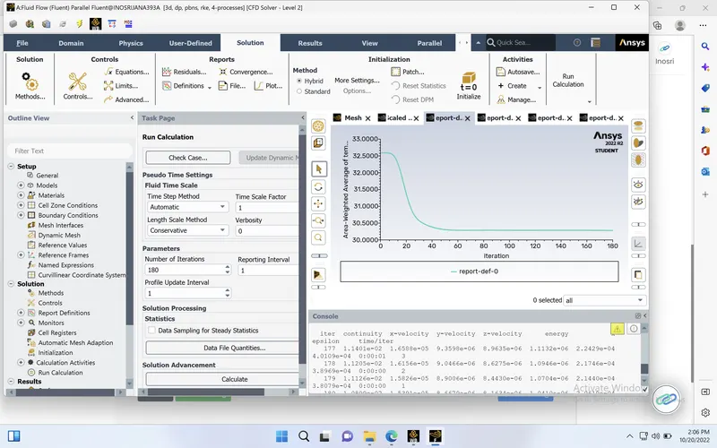
Area weighted avg of temp at the outlet:

Standard deviation of temp at the outlet:

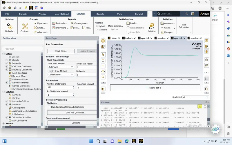
Area weighted avg of velocity at the outlet:

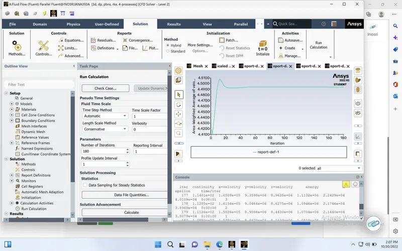
Result analysis:

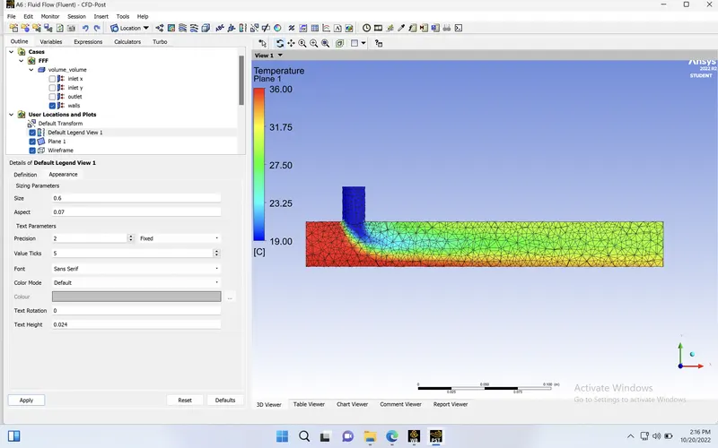
Velocity and temperature contour plots on the cut planes along and across the pipe

Temperature Distribution:plane 1

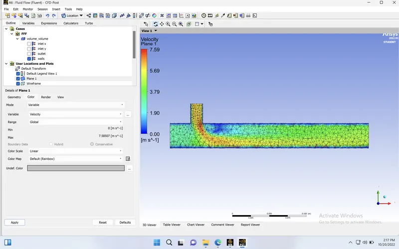
Velocity distribution:plane1

Velocity and temperature line plots along and across the length of the pipe:

Temperature line plots along length of the pipe:

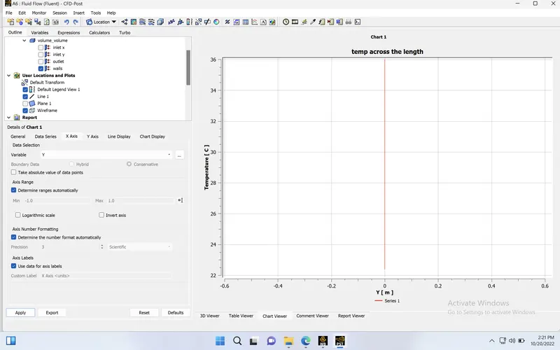
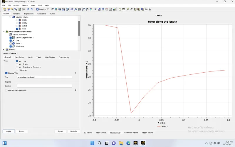Temperature line plots across length of the pipe:

Velocity line plots along length of the pipe:

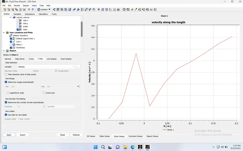
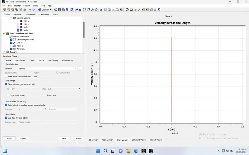
Velocity line plots along length of the pipe:

Long mixing tee with a hot inlet velocity of 3m/s : k-epsilon model: Momentum ratio of 4

solution:

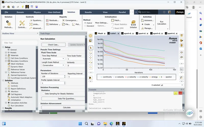
Residuals of governing and transport equations :

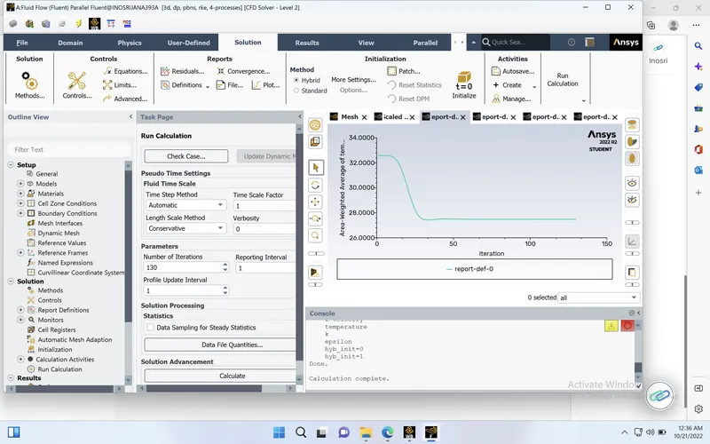
Area weighted avg of temp at the outlet:

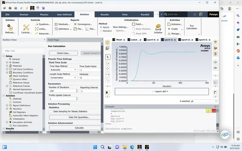
Standard deviation of temp at the outlet:

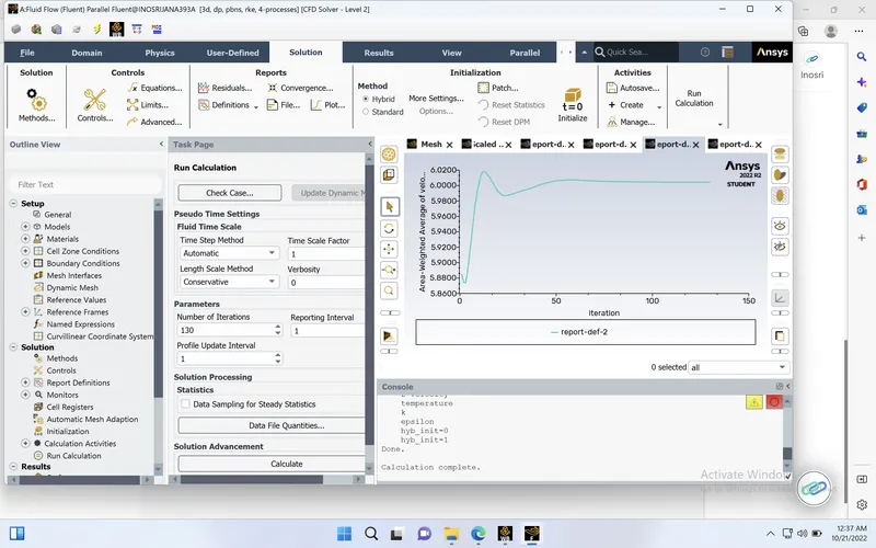
Area weighted avg of velocity at the outlet:

Result analysis:

Velocity and temperature contour plots on the cut planes along and across the pipe

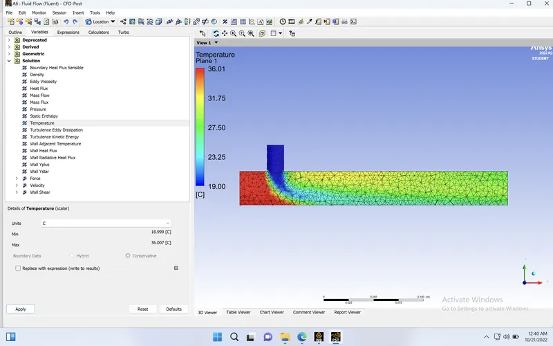
Temperature Distribution:plane1

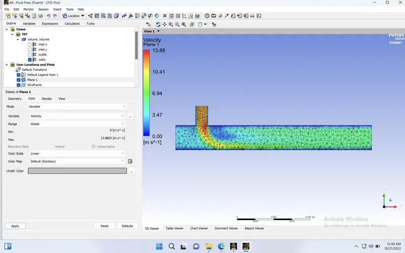
Velocity distribution:plane1

Velocity and temperature line plots along and across the length of the pipe:

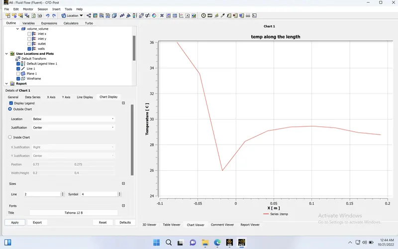
Temperature line plots along length of the pipe:

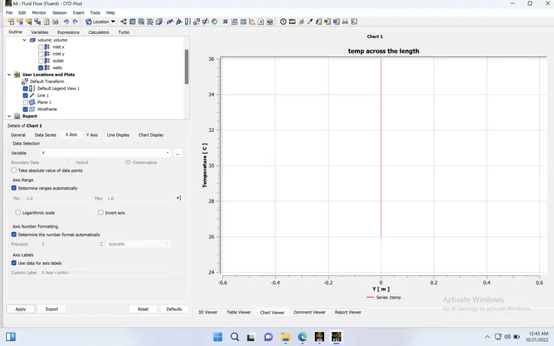
Temperature line plots across length of the pipe:

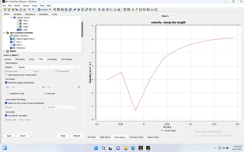
Velocity line plots along length of the pipe:

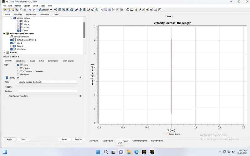
Velocity line plots across length of the pipe:

Comparision of the following values from the 2 cases.

1. Cell count
2. Average outlet temperature
3. Number of iterations for convergence

Cases	Cell count	Average outlet temperature	Number of iterations for convergence
Short mixing tee with a hot inlet velocity of 3m/s. Momentum ratio of 2 k-omega SST	12691	30.26 0C	170
Short mixing tee with a hot inlet velocity of 3m/s. Momentum ratio of 2 k-epsilon	12691	30.24 0C	150
Short mixing tee with a hot inlet velocity of 3m/s. Momentum ratio of 4 k-epsilon	12691	27.53 0C	130
Long mixing tee with a hot inlet velocity of 3m/s. Momentum ratio of 2 k-epsilon	15788	30.28 0C	180
Long mixing tee with a hot inlet velocity of 3m/s. Momentum ratio of 4 k-epsilon	15788	27.48 0C	130

Analytical solution:

(K-epsilon)

short mixing tee momentum ratio 2:

mass flow rate of hot fluid (m_h)=0.0032 kg/s

mass flow rate of cold fluid (m_h)=0.0016 kg/s

T_(mixture)=(0.0032*36+0.0016*19)/(0.0032+0.0016)=30.33⁰C

(close to simulation value 30.24⁰C)

short mixing tee momentum ratio 4:

mass flow rate of hot fluid (m_h)=0.0032 kg/s

mass flow rate of cold fluid (m_h)=0.0032 kg/s

T_(mixture)=(0.0032*36+0.0032*19)/(0.0032+0.0032)=27.53⁰C

long mixing tee momentum ratio 2:

mass flow rate of hot fluid (m_h)=0.0032 kg/s

mass flow rate of cold fluid (m_h)=0.0016 kg/s

T_(mixture)=(0.0032*36+0.0016*19)/(0.0032+0.0016)=30.33⁰C

(close to simulation value 30.28⁰C)

long mixing tee momentum ratio 4:

mass flow rate of hot fluid (m_h)=0.0032 kg/s

mass flow rate of cold fluid (m_h)=0.0032 kg/s

T_(mixture)=(0.0032*36+0.0032*19)/(0.0032+0.0032)=27.50⁰C

(close to simulation value 27.48⁰C)

Mesh independent study :

• Short mixing tee with a hot inlet velocity of 3m/s.
• Momentum ratio of 2
• k-epsilon

Mesh size	Elements	Nodes	Average outlet temperature	Number of iterations for convergence
.005 m	14361	3160	30.240C	177
.003 m	40088	8397	30.27 0C	250

Average outlet temerature is nearly same in both cases.So it is mesh independent.

k-epsilon suitability:

K epsilon is best suited for flow away from the wall, say free surface flow region, whereas k-omega model is best suited for near the wall flow region, where adverse pressure gradient is developed.It is one of the most commonly used turbulence model based on RANS(Reynolds Averaged Navier- Stockes) equation but it doesnt perform well in case of large adverse pressure gradients.It is a two equation model. The first transported variable is turbulent kinetic energy k. the second trasnported cariable is turbulent dissipation ε , which is a variable thta determines the scale of turbulence.When comparing the K-epsilon and K-omega model for flow through mixing tee we can find that the simulation is faster in case of k epsilon model.Covergence can be reached easily .

The effect of length and momentum ratio on results:

Irrespective of the length of mixing tee the outlet temperature is nearly same.

Increasing the momentum ratio increases the temperature of cold inlet air therefore outlet temp get reduced.Therefore less momentum ratio is preferred.

Conclusion:

Steady-state simulations to compare the mixing effectiveness are succesfully done.