Week 1- Mixing Tee
THERMAL MIXING PHENOMENA IN T- JUNCTION USING ANSYS FLUENT 2021 R1
SUBMITTED BY: VINITHA JOHNY
The thermal mixing phenomena have been investigated in 2 test case scenarios.Steady-state simulations are set up to compare the mixing effectiveness when hot inlet temperature is 360C & the Cold inlet is at 190C.
- Case 1
- Short mixing tee with a hot inlet velocity of 3m/s.
- Momentum ratio of 2, 4.
- Case 2
- Long mixing tee with a hot inlet velocity of 3m/s.
- Momentum ratio of 2, 4.
Momentum ratio = velocity at cold inlet / velocity at hot inlet
INTRODUCTION
Mixing of air at an isothermal condition in a T junction in the horizontal plane is carried out. Experiments have been carried out by varying the flow rates in the main and branch pipe. The mixing of air from both the pipes can be tackled by Reynolds averaged Navier-stokes equation(RANS).
CASE 1 SHORT MIXING TEE
The objective of the project is to establish a work flow in a mixing tee pipe using ANSYS FLUENT. The basic solid model is imported to space claim where the fluid volume (1.7944e-004 ) is extracted using edge method before analysing.
|
Surface |
Area of the surface |
Length in metres |
|
Inlet x |
0.19238 m |
|
|
Inlet y |
6.0099e-002 m |
|
|
Outlet |
3.3876e-002m |
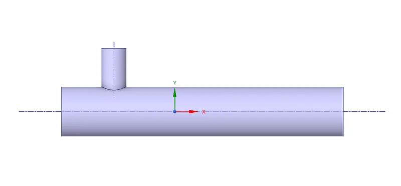
Fig.1.Basic solid model of mixing T
The simulations were carried out for only one half of the geometry, which is possible in the case of isothermal steady-state flow simulations, where buoyancy effects are neglected.
In the meshing part, the boundaries are named as Inlet x, Inlet y, Outlet, and walls. The details regarding the mesh is not altered much to get a quadrilateral basic mesh. The geometry is then cut into 2 halves for further investigation.
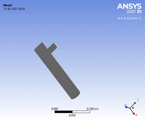
Fig.2.Geometry to be investigated
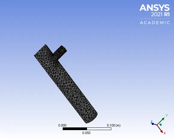
Fig.3.quadrilateral mesh
The effectiveness of meshing is obtained through elementary statistics. The quality of the mesh is obtained using the mesh metric option. Every meshing should meet a minimum threshold quality. The histogram below gives a minimum quality of 38% and a maximum quality of 100%, which is moderately fine to be investigated by Ansys.
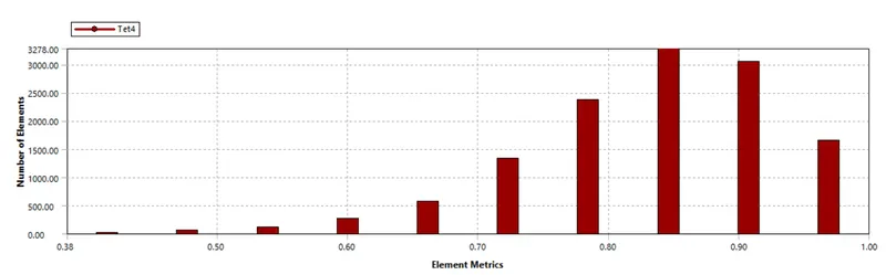
Fig.4.Element quality graph
|
Mesh metric |
Element quality |
|
Min |
0.38441 |
|
Max |
0.9999 |
|
Average |
0.83448 |
|
Standard deviation |
9.5868e-002 |
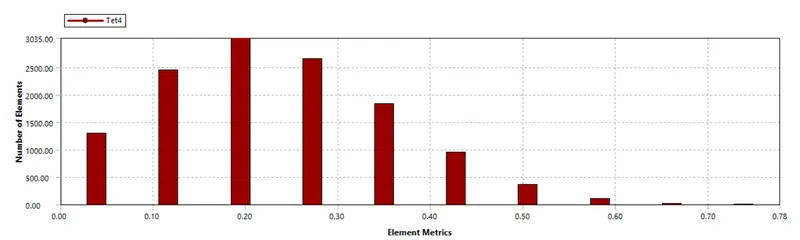
Fig.6.Skewness
|
Mesh metric |
Skewness |
|
Min |
9.9774e-005 |
|
Max |
0.77736 |
|
Average |
0.2317 |
|
Standard Deviation |
0.1219 |
The physics behind the analysis is pressure based with a turbulence model of K epsilon in the bulk of the flow. The velocity formulation is absolute with a steady time. We are also keen to solve for the temperature.
The boundary conditions are given as input where the Inlet x has the type velocity intake with a velocity magnitude of 3m/s. The thermal temperature is set to 25 degree celcius. The velocity magnitude of Inlet y is set to 10m/s.
Reports based on the Area weighted area and surface deviation of the outlet is obtained for the temperature variable. The console is run after 10,150 and 250 iterations respectively to obtain the graphs.
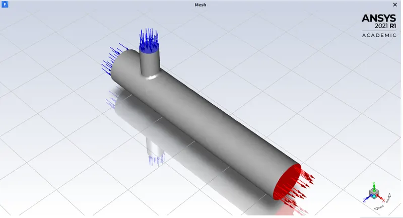
Fig.7.Mesh model representing the inlets and outlet
|
Surface |
Velocity magnitude m/s |
Temperature |
|
Hot inlet |
3m/s |
36 |
|
Cold inlet |
6m/s, 12m/s |
19 |
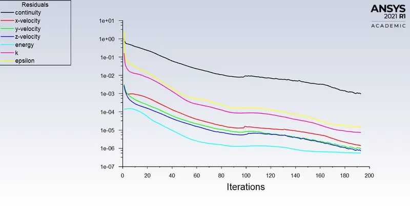
Fig.8. Graph of residuals after 193 iterations
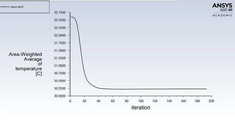
Fig.9.Graph of Area-weighted average of temperature after 193 iterations
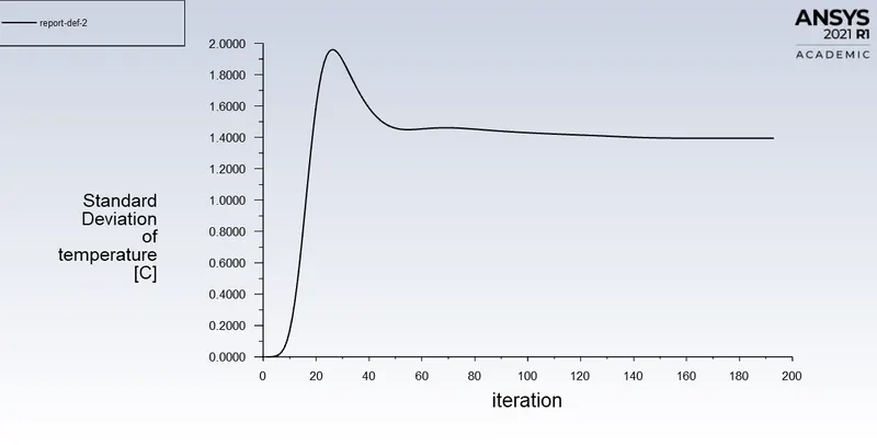
Fig.10.Graph of standard deviation of temperature[C]
Results
The velocity distribution and pressure distribution is done as follows.
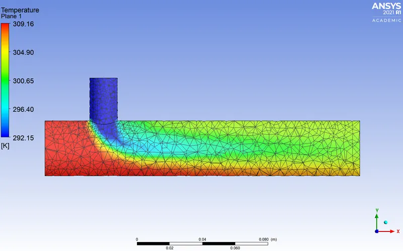
Fig.11.Temperature distribution along the pipe
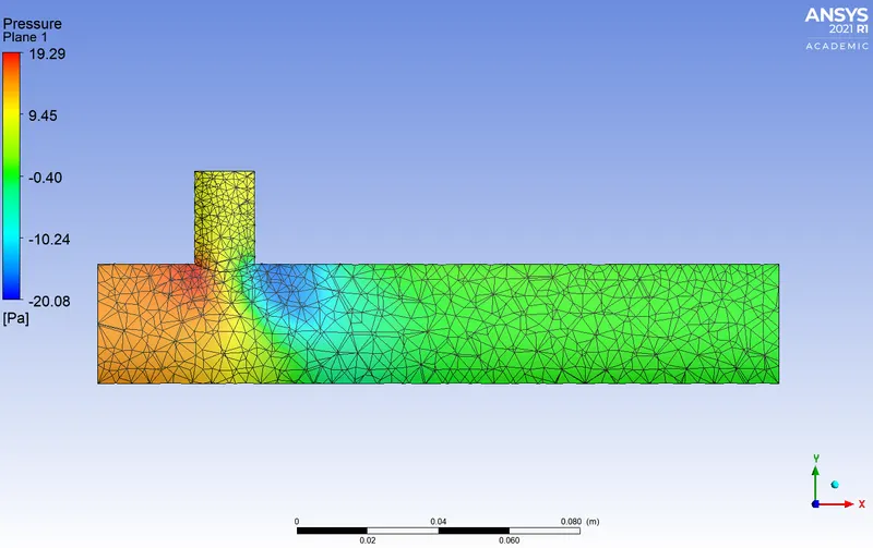
Fig.12.Pressure distribution along the pipe
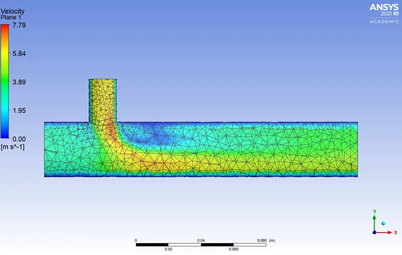
Fig.13.velocity along the pipe
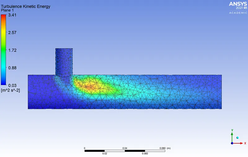
Fig.14.Turbulence kinetic energy along the pipe
- The Standard Deviation of the outlet is calculated. A high value of SD denotes poor mixing and a low value suggests a relatively good mixing.
- The temperature mixing takes place to a relatively greater extend along the x axis which reduces the outlet temperature to 304.9 K.
- The inlet x is under a relatively higher pressure compared to the outlet. The blind spot near the inlet y is a low pressure area.
- The pipe has a guage pressure of 0 pascal
- The velocity is very low along the walls of the pipe.
- The turbulence kinetic energy is high at the part of mixing and very low in the rest of the pipe.
CASE 2 LONG MIXING TEE
The objective of the project is to establish a work flow in a long mixing tee pipe using ANSYS FLUENT. The basic solid model is imported to space claim where the fluid volume (2.479e-004 ) is extracted using edge method before analysing.
|
Surface |
Area of the surface |
Length in metres |
|
Inlet x |
0.26833 m |
|
|
Inlet y |
6.0099e-002 m |
|
|
Outlet |
3.3876e-002m |
The simulations were carried out for only one half of the geometry, which is possible in the case of isothermal steady-state flow simulations, where buoyancy effects are neglected.
In the meshing part, the boundaries are named as Inlet x, Inlet y, Outlet, and walls. The details regarding the mesh is not altered much to get a quadrilateral basic mesh. The geometry is then cut into 2 halves for further investigation.
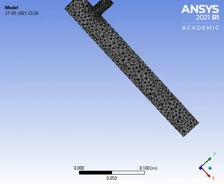
Fig.3.quadrilateral mesh
The effectiveness of meshing is obtained through elementary statistics. The quality of the mesh is obtained using the mesh metric option. Every meshing should meet a minimum threshold quality.The histogram below gives a minimum quality of 36;lllllllllll% and a maximum quality of 100%, which is moderately fine to be investigated by Ansys.
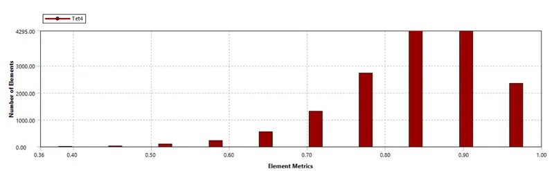
Fig.4.Element quality graph
|
Mesh metric |
Element quality |
|
Min |
0.35772 |
|
Max |
0.99984 |
|
Average |
0.84156 |
|
Standard deviation |
9.173e-002 |
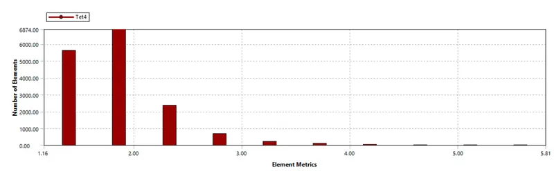
Fig.5.Aspect Ratio graph
|
Mesh metric |
Aspect ratio |
|
Min |
1.1629 |
|
Max |
5.8134 |
|
Average |
1.8379 |
|
Standard Deviation |
0.43227 |
The physics behind the analysis is pressure based with a turbulence model of K epsilon in the bulk of the flow. The velocity formulation is absolute with a steady time. We are also keen to solve for the temperature.
The boundary conditions are given as input where the Inlet x has the type velocity intake with a velocity magnitude of 3m/s. The thermal temperature is set to 36 . The velocity magnitude of Inlet y is set to 6m/s with temperature 19
Reports based on the Area weighted area and surface deviation of the outlet is obtained for the temperature variable. The console is run after 10,150 and 250 iterations respectively until the graph converges
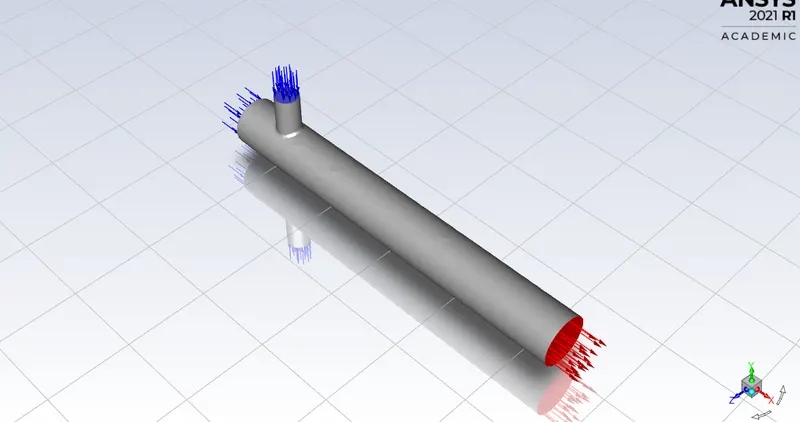
Fig.7.Mesh model representing the inlets and outlet
|
Surface |
Velocity magnitude m/s |
Temperature |
|
Hot inlet |
3m/s |
36 |
|
Cold inlet |
6m/s, 12m/s |
19 |
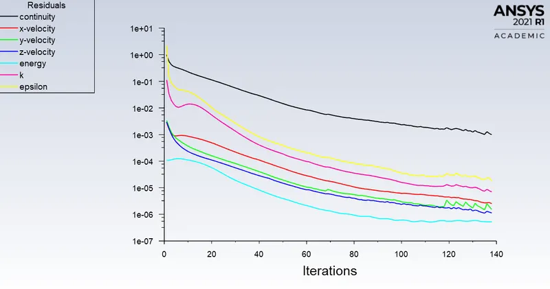
Fig.8. Graph of residuals after 138 iterations
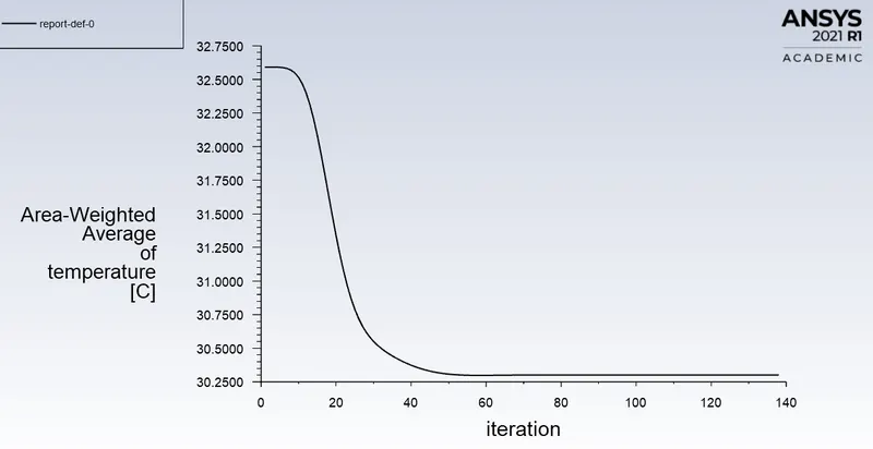
Fig.9.Graph of Area-weighted average of temperature after 138 iterations
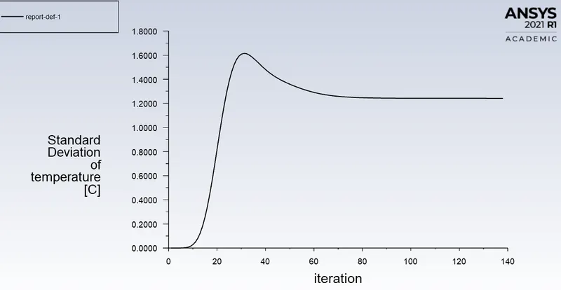
Fig.10.Graph of standard deviation of temperature[C]
Results
The velocity distribution and pressure distribution is done as follows.
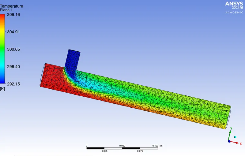
Fig.11.Temperature distribution along the pipe
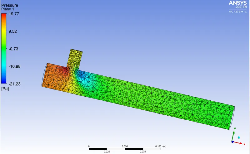
Fig.12.Pressure distribution along the pipe
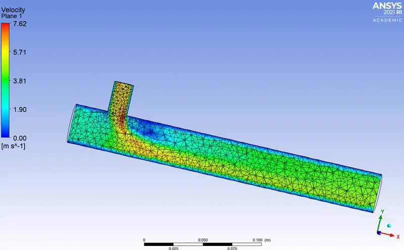
Fig.13.velocity along the pipe
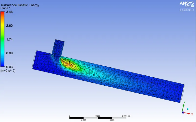
Fig.14.Turbulence kinetic energy along the pipe
- The Standard Deviation of the outlet is calculated. A high value of SD denotes poor mixing and a low value suggests a relatively good mixing.
- The temperature mixing takes place to a relatively greater extend along the x axis. The hot inlet air mixes with the cold inlet air to reduce the overall temperature to 300.6 K at the outlet.
- The pressure throughout the pipe is almost constant after mixing.
- The velocity of the air is high along the walls of the pipe.
- The turbulence kinetic energy is high at the part of mixing and very low in the rest of the pipe.
RELATIVE EVALUATION
|
CASE 1short |
CASE 2 long |
|
|
Cell count |
12663 |
15802 |
|
Average outlet temperature |
304.9 K |
300.6 K |
|
No of iterations for convergence |
193 |
138 |
|
CASE 1 short |
CASE 2 long |
|
|
Iterations |
193 |
138 |
|
X velocity |
1.405e-06 |
2.52e-06 |
|
Y velocity |
9.182e-07 |
1.546e-06 |
|
Z velocity |
7.250e-02 |
1.133e-06 |
|
Energy |
5.521e-07 |
5.2522e-07 |
|
K |
7.338e-06 |
6.981e-06 |