Week 1- Mixing Tee

Aim:

To simulate the air flow through the mixing tee and to set up steady-state simulations to compare the mixing effectiveness when hot inlet temperature is 36⁰C & the Cold inlet is at 19⁰C.

Objective:

In this challenge we have to find four cases.

1. Case 1
   • Short mixing tee with a hot inlet velocity of 3m/s. Temperature of the hot tee =36c and temperature of the cold tee = 19c
   • Momentum ratio of 2. (Velocity hot tee = 3m/s, velocity cold tee =6m/s)
2. Case 2
   • Short mixing tee with a hot inlet velocity of 3m/s. Temperature of the hot tee =36c and temperature of the cold tee = 19c
   • Momentum ratio of 4. (Velocity hot tee = 3m/s, velocity cold tee =12m/s)
3. Case 3
   • Long mixing tee with a hot inlet velocity of 3m/s. Temperature of the hot tee =36c and temperature of the cold tee = 19c
   • Momentum ratio of 2. (Velocity hot tee = 3m/s, velocity cold tee =6m/s)
4. Case 4
   • Long mixing tee with a hot inlet velocity of 3m/s. Temperature of the hot tee =36c and temperature of the cold tee = 19c
   • Momentum ratio of 4. (Velocity hot tee = 3m/s, velocity cold tee =12m/s)

Formula:

Momentum ratio = velocity at cold inlet / velocity at hot inlet

Step by step procedure of ANSYS FLUENT:

• Geometry
• Meshing
• Set up
• Solution
• Result

Above the five steps are major procedure in ansys fluent. We have to follow these steps in ANSYS FLUENT. Each and every case we have follow these steps.

Case 1:

We have to open the ANSYS FLUENT workbench and then we have to click fluent flow. It will open the pop-up box. These pop box having five major steps Geometry, Meshing, Set up, Solution, Result. We want to follow these steps. Because ansys fluent is a step-by-step procedure.

First step we have to upload the given short mixing tee in ansys fluent workbench by using geometry (space claim option). Once you uploaded the geometry go to prepare option and then we have click volume extract option and the click select edges option and then we should select the volumes and click the green tick symbol the geometry will showing the volume surface and remaining surface and then go to shell right click and then click supress to physics option then the geometry will get ready for the next process. Once complete the geometry model the image will show below like this both case 1 & 2.

Second step is meshing process we have to upload the prepared geometry in mesh option for case 1 & 2. And then right click to generate mesh option the mesh will be generated and then click the face option right click create named selection option to create name inlet-y, inlet-x, outlet, walls. Once complete the meshing process after that we have to move next process. Below the image is denoted case 1 & 2 mesh image.

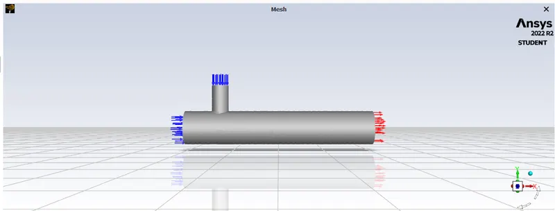
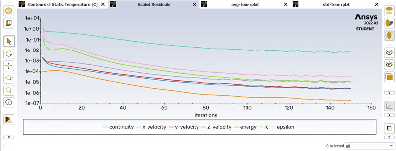
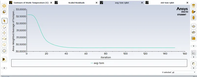
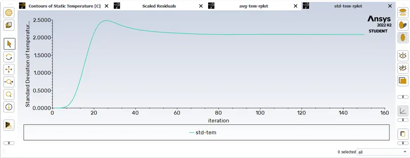
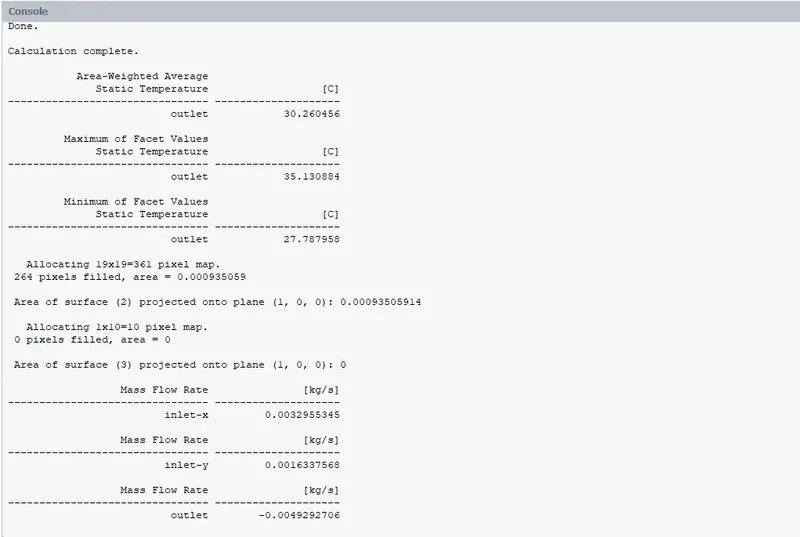
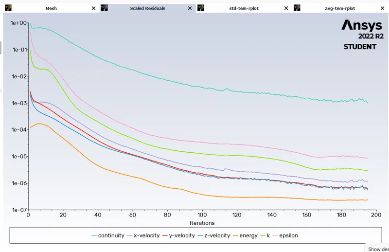
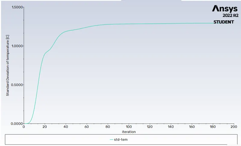
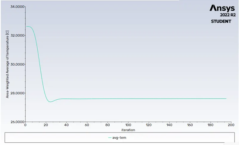
Next, we have to create surface report click on the solutions go to report definitions – new – surface report- area – area-weighted average as well as we have to create standard deviation of outlet temperature. Once complete this process next we have to move simulation process we should initialize the flow field by clicking on t=0 initialize option. And then we have to give iteration around 150 and then just click run calculation. If the iteration is not converged, we should give 300 iterations. Once complete the iteration converge process, we get the average temperature plot and standard deviation plots.

Case 1 & 2 set-up image:

Case 1 residuals:

Case 1 Avg temperature:

Case 1 standard ddeviation temperature:

Solution:

Some solutions completed in set-up option also. So we have to move next step of the results.

Case 2 residual plot:

Case 2 standared deviation temperature plot:

Case 2 Area-weighted average of temperature plot:

Solution:

Some solutions completed in set-up option also. So we have to move next step of the results.

Case 3 & 4 geometry:

Case 3&4:

We have to open the ANSYS FLUENT workbench and then we have to click fluent flow. It will open the pop-up box. These pop box having five major steps Geometry, Meshing, Set up, Solution, Result. We want to follow these steps. Because ansys fluent is a step-by-step procedure.

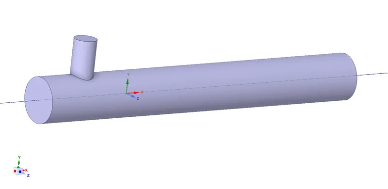
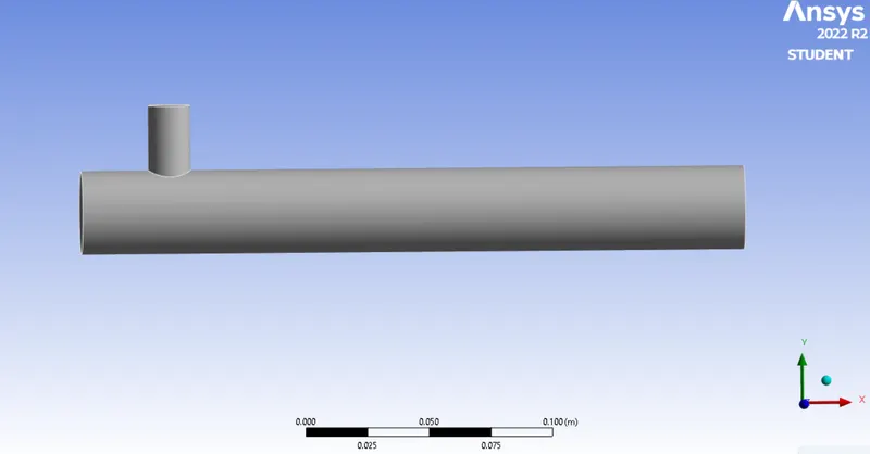
First step we have to upload the given long mixing tee in ansys fluent workbench by using geometry (space claim option). Once you uploaded the geometry go to prepare option and then we have click volume extract option we should select the volumes and click the green tick symbol the geometry will showing the volume surface and remaining surface and then go to shell right click and then click supress to physics option then the geometry will get ready for the next process. Once complete the geometry model the image will show below like this.

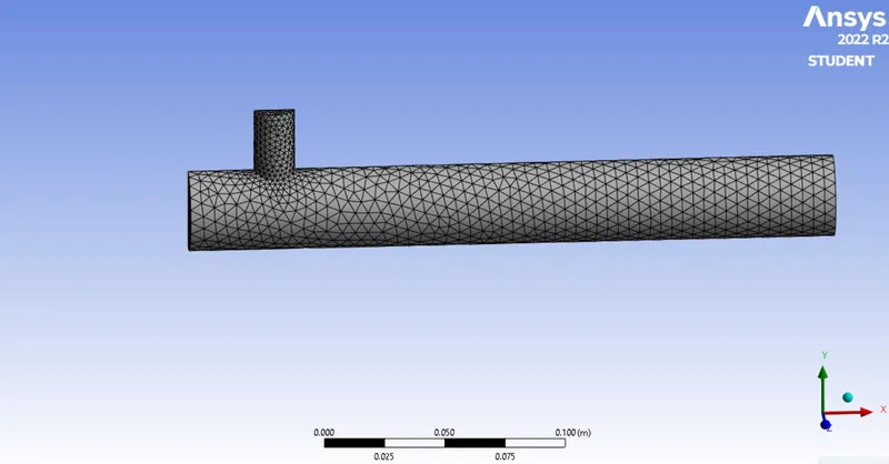
Second step is meshing process we have to upload the prepared geometry in mesh option for case 1 & 2. And then right click to generate mesh option the mesh will be generated and then click the face option right click create named selection option to create name inlet-y, inlet-x, outlet, walls. Once complete the meshing process after that we have to move next process. Below the image is denoted case 1 & 2 mesh image.

Right click on the set-up, opens the fluent launcher. In the fluent launcher we have to select 3D, double precision and select the number of cores and we have to give 4 as per the user configuration system. And then we have to defined some simulation definitions like

Type: Pressure based

Velocity formulation: Absolute

Time: Steady

Next go to physics tab click to turn on Energy and then go to viscous select k-epsilon.

Next go to materials we have to select air it is a default material and the material type is fluid.

Next go to cell zone conditions select the volume and it should show default option fluid click that option.

Next step is we have to define boundary condition as given below,

1. Case 3
   • Long mixing tee with a hot inlet velocity of 3m/s. Temperature of the hot tee =36c and temperature of the cold tee = 19c
   • Momentum ratio of 2. (Velocity hot tee = 3m/s, velocity cold tee =12m/s)
2. Case 4
   • Long mixing tee with a hot inlet velocity of 3m/s. Temperature of the hot tee =36c and temperature of the cold tee = 19c
   • Momentum ratio of 4. (Velocity hot tee = 3m/s, velocity cold tee =12m/s)

Outlet should be the pressure outlet.

Next, we have to create surface report click on the solutions go to report definitions – new – surface report- area – area-weighted average as well as we have to create standard deviation of outlet temperature. Once complete this process next we have to move simulation process we should initialize the flow field by clicking on t=0 initialize option. And then we have to give iteration around 150 and then just click run calculation. If the iteration is not converged, we should give 300 iterations. Once complete the iteration converge process, we get the average temperature plot and standard deviation plots.

Case 3 standared deviation temperature plot:

Case 3 Area-weighted average of temperature plot:

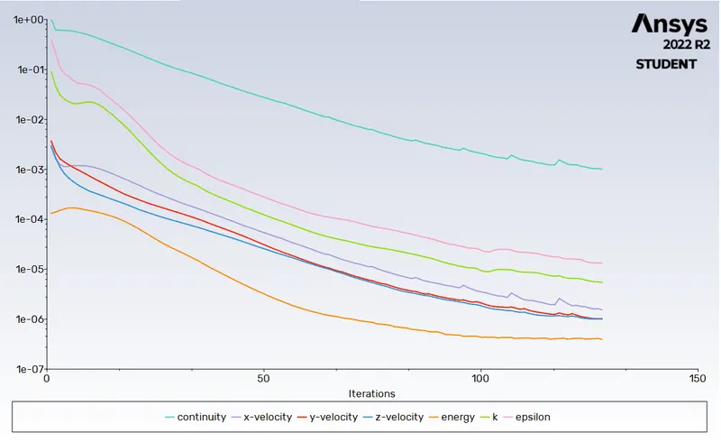
Case 4 residual plot:

Case 4 Area-weighted average of temperature plot:

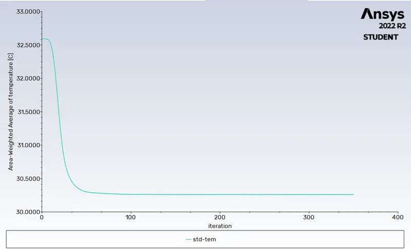
Case 4 standared deviation temperature plot:

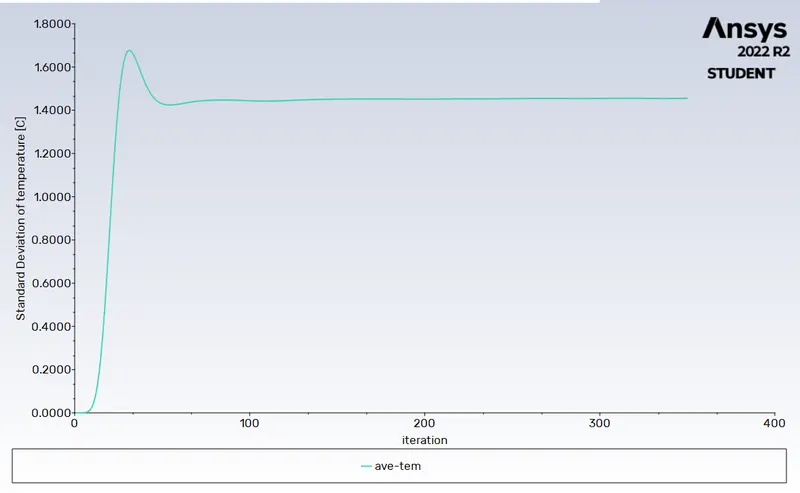
Result:

Result option is nothing but post processing option. We should open the result option it will open. It will show wireframe mode of the geometry and then we can create plane by using location option. Selecting the vector option, the plane will create velocity vector contour plot.

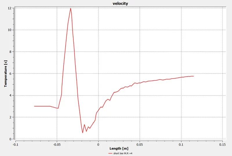
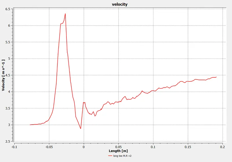
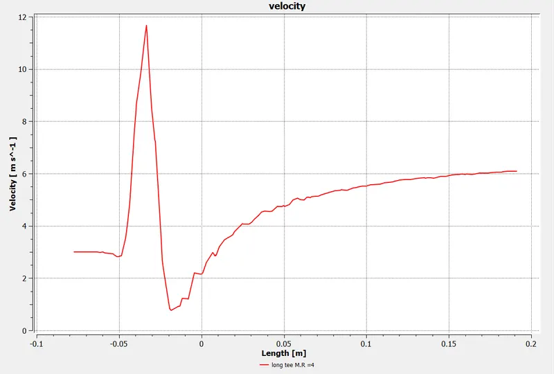
Again, go to location we can create line. The line will cut the plane of the central axis and the line is used to collect the temperature and velocity data.

Similarly go to ANSYS FLUENT workbench we have to right click and get duplicate for case 2 & 4

Case 1 velocity magnitude contour plot:

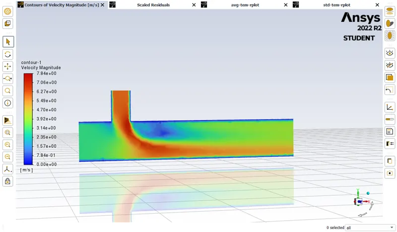
Case 2 velocity magnitude contour plot:

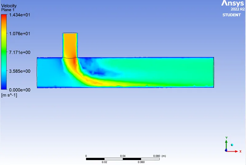
Case 3 velocity magnitude contour plot:

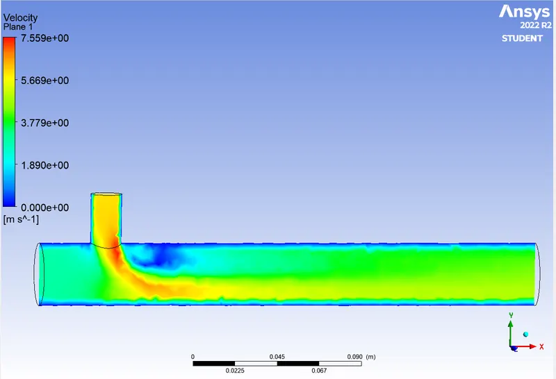
Case 4 velocity magnitude contour plot:

Case 1 temperature magnitude contour plot:

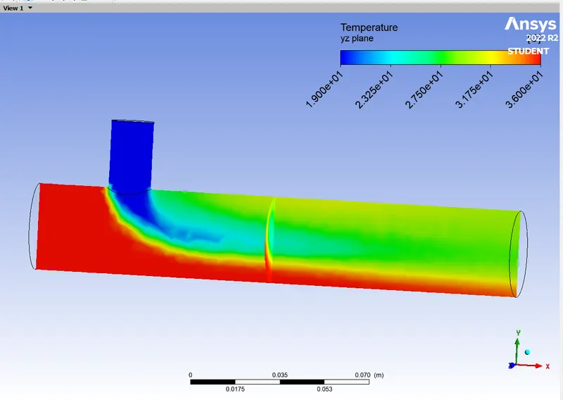
Case 2 temperature magnitude contour plot:

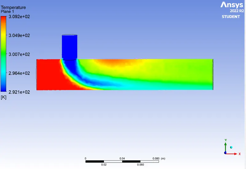
Case 3 temperature magnitude contour plot:

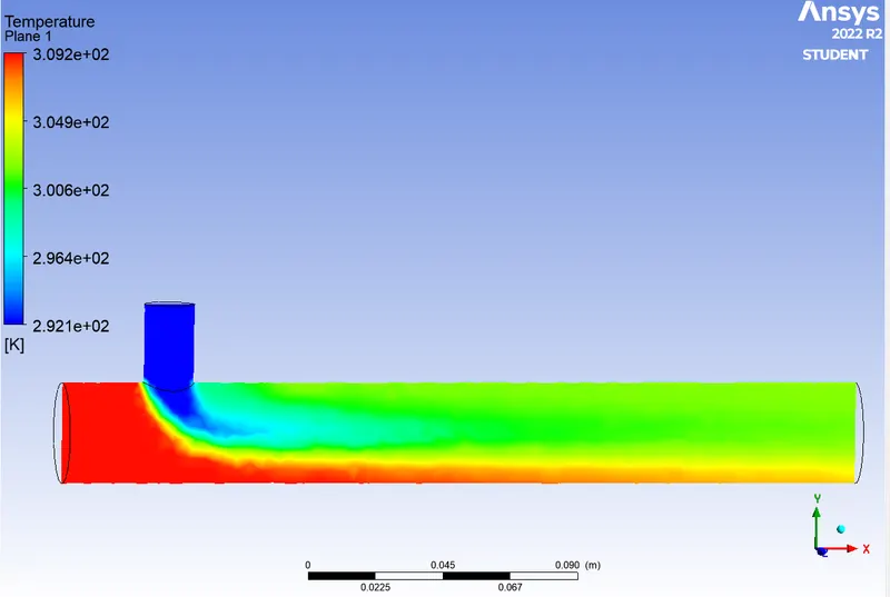
Case 4 temperature magnitude contour plot:

Result:

Result option is nothing but post processing option. We should open the result option it will open. It will show wireframe mode of the geometry and then we can create plane by using location option. Selecting the vector option, the plane will create velocity vector contour plot.

Again, go to location we can create line. The line will cut the plane of the central axis and the line is used to collect the temperature and velocity data.

Similarly go to ANSYS FLUENT workbench we have to right click and get duplicate for case 2&4.

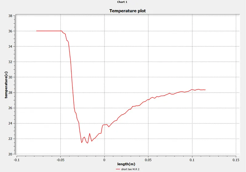
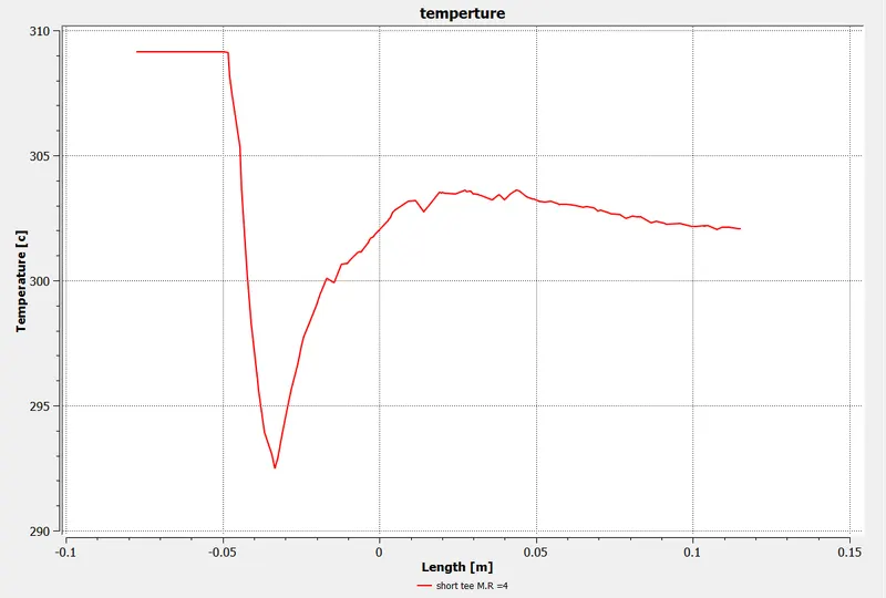
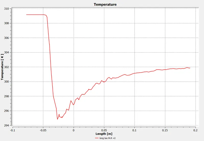
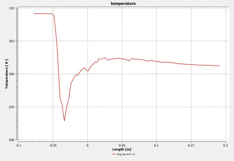
Go to chart option create velocity and temperature charts.

Case 1 temperature chart:

Case 2 temperature chart:

Case 3 temperature chart:

Case 4 temperature chart:

Result:

Result option is nothing but post processing option. We should open the result option it will open. It will show wireframe mode of the geometry and then we can create plane by using location option. Selecting the vector option, the plane will create velocity vector contour plot.

Case 1 vector contour plot:

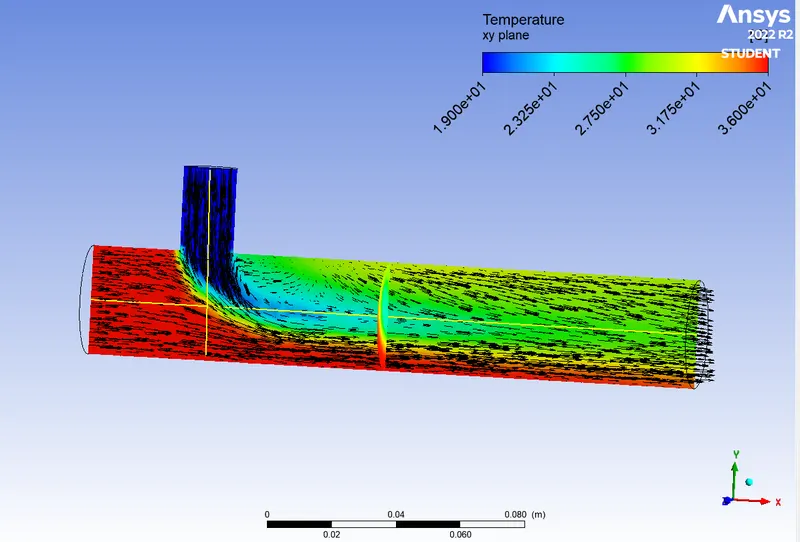
Case 2 vector contour:

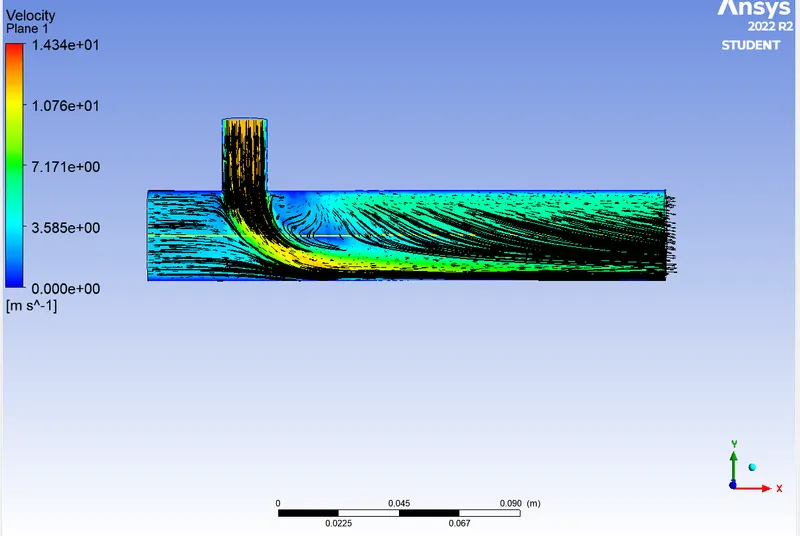
Case 3 vector contour:

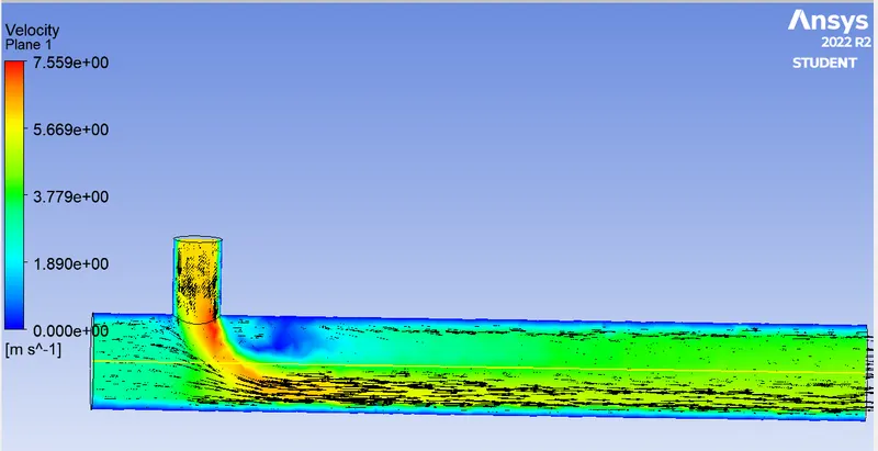
Case 4 vector contour:

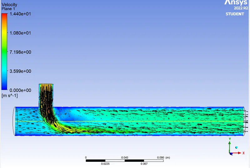
Case 1 velocity chart:

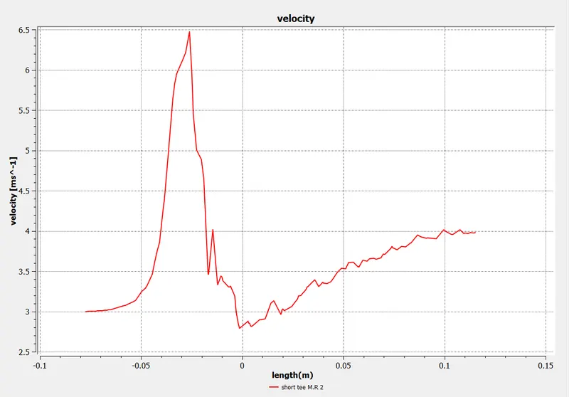
Case 2 velocity chart:

Case 3 vector chart:

Case 4 velocity chart:

Inferance comparison table:

case 1 case 2 case 3 case 4

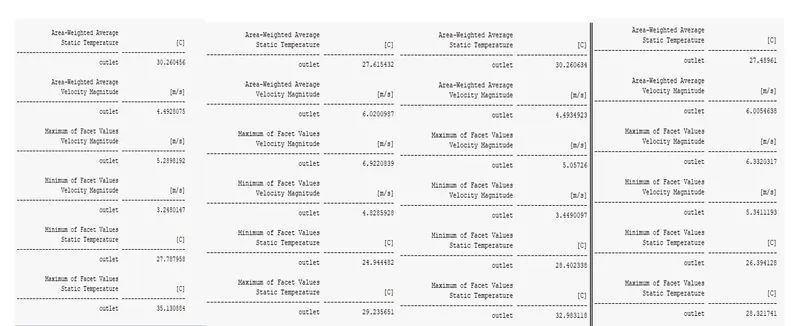
cell count:

case 1: 15727 case 2: 15727 case 3: 39792 case 4: 39792

Conclusion:
Finally, the results we obtained from all 4 cases and its comparison visually from the graphs and contours we can say that case 2 is better compare to 4 cases. We have to give the 3mm mesh. So let we see in the four case almost similar to the numerical values. Case 2 is easily converged in 132 iterations so the case 2 is better compare to other cases.

Reference:

https://www.sciencedirect.com/science/article/pii/S0142727X21000916

https://www.sciencedirect.com/science/article/pii/S0029549309005676