Week 1- Mixing Tee

MIXING TEE

Aim:-

To set up steady-state simulations to compare the mixing effectiveness when the hot inlet temperature is 36⁰C & the Cold inlet is 19⁰C. For that purpose, two versions of the mixing tee are created. One of them is longer than the other.

Run the simulations for different values of the Momentum Ratio (2 & 4).

1. Case 1
   • Short mixing tee with a hot inlet velocity of 3m/s.
   • Momentum ratios of 2 and 4.
2. Case 2
   • Long mixing tee with a hot inlet velocity of 3m/s.
   • Momentum ratios of 2 and 4.

Also, compare the following values from both the cases

1. Cell count
2. Average outlet temperature
3. Number of iterations for convergence

Theory:-

Modern industrial processes almost always involves some form of mixing. A mixing tee is a type of mixing mechanism. Mixing Tees utilizes a specifically engineered internal geometry to efficiently mix two fluid streams into one combined stream. Mixing tees are widely used in the petrochemical, HVAC industry, etc. in which two fluid streams with different physical and/or chemical properties mix together.

Turbulent mixing of fluids of different temperatures in T-junction geometries became of significant importance in the field of nuclear reactor safety since it can lead to highly transient temperature fluctuations at the adjacent pipe walls, cyclic thermal stresses in the pipe walls, and consequently to thermal fatigue and failure of the pipeline. In general, thermal striping and mixing are challenging to predict by using standard CFD simulation and turbulence modeling approaches.

Here hot air flowing in the main pipe is mixed with cold air flowing through a tee. The standard deviation of temperature is computed to quantify the degree of mixing. We use the given momentum ratio to determine the cold air temperature. Momentum ratio is defined as the ratio of velocity at the cold inlet to the velocity at the hot inlet.

Modeling and Solving Approach:-

• The workflow in Ansys fluent is as follows

  Geometry -> Mesh -> Setup -> Solution -> Results

• First, we need to create or import the required geometry and edit it in Spaceclaim.
• The next step is mesh generation
• We then set up the problem according to the challenge statement. Boundary conditions and which model to be used are decided here.
• After running the iterations, we can use post processor to obtain necessary plots and graphs as results.
• The procedure followed for one case will be explained in detail as it is the same for other cases.

Preprocessing:-

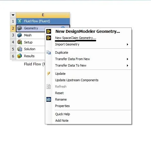
• First, we need to open Spaceclaim by right-clicking the Geometry section.

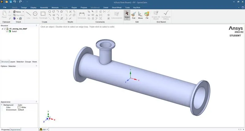
• Import the CAD model into the Spaceclaim.
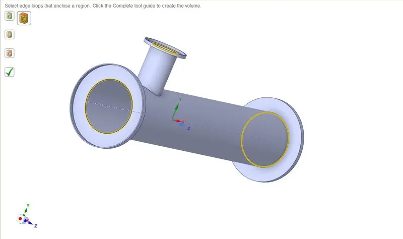
• Use the Volume Extract tool and then extract the fluid volumes the solid part is not required.
• We can use Suppress for the physics option so that the solid body won't interfere with our simulations.

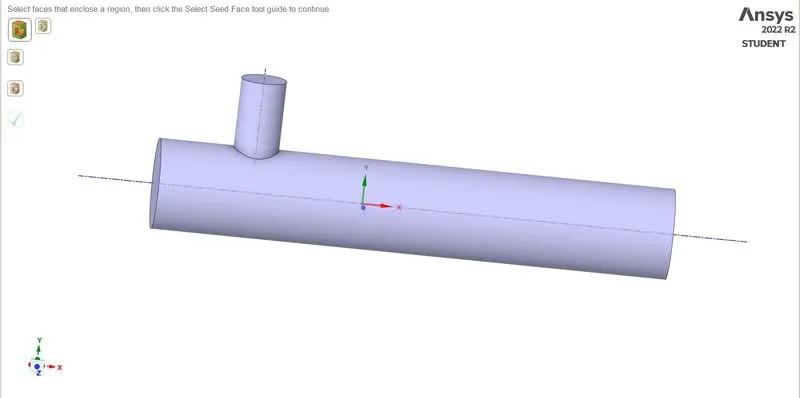
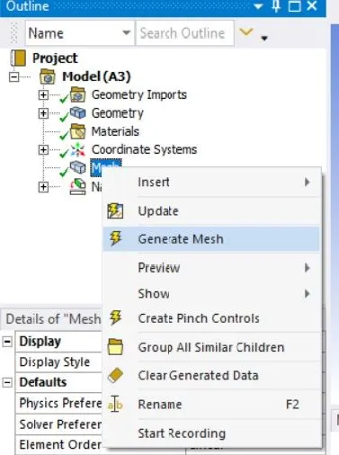
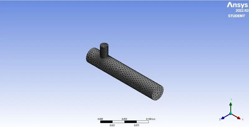
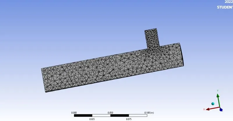
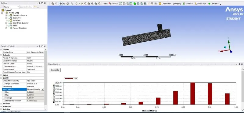
• The next step is to generate mesh on the fluid volume extracted. In this case, we can use Generate Mesh option. The element size was given as 3mm.

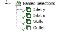
• Now we need to name the boundaries. Select the face and right-click. Choose the Create Named Selection.

• Check the quality of mesh created in mesh matric. Here mesh quality is above 30% or 0.3 and we can use this mesh for further study.

Solver setup:-

Fluent Set up

1.	Solver	Steady-state
2.	Energy	ON
3.	Turbulence Model	k-epsilon / k-omega
4.	Inlet	Velocity inlet
5.	Outlet	Pressure outlet - Atm pressure
6.	Hot inlet velocity	3 m/s
7.	Cold inlet velocity	6 m/s and 12 m/s
8.	Hot inlet temperature	36 C
9.	Cold inlet temperature	19 C

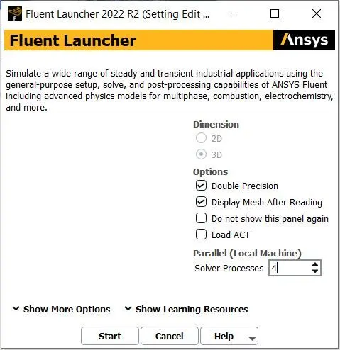
• Open the Setup and check whether the mesh is of good quality or not. We can also change units before proceeding.
• Select model and boundary conditions as given above.
• For the material part, the fluid is defined as air
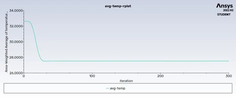
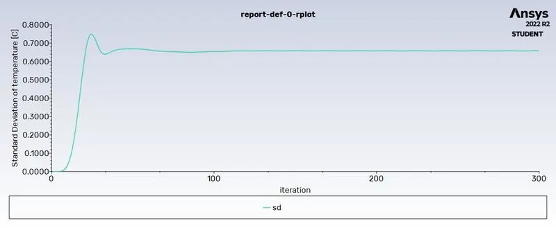
• Create 2 report definitions for Average temperature (Area weighted average) and Standard deviation at the outlet.
• The next step is to do the initialization using the Hybrid method.
• We can decide the number of iterations next. We'll start with 150 iterations in this case.

Post-processing:-

• Once the iterations are done, we can move on to the post-processing part. Select the Results
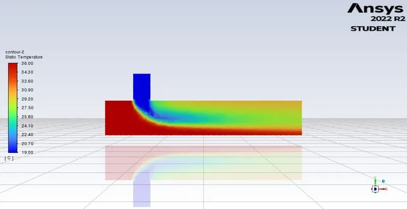
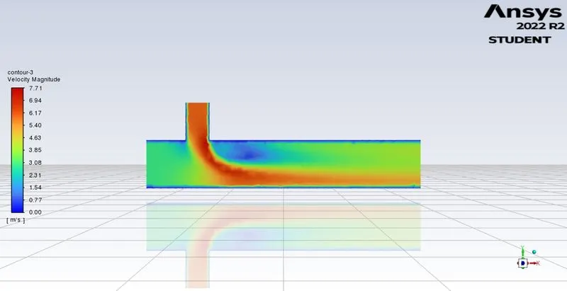
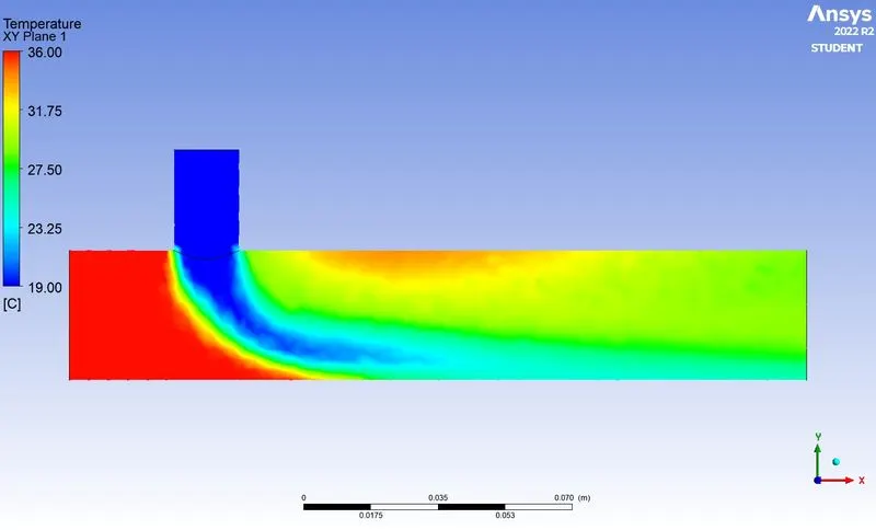
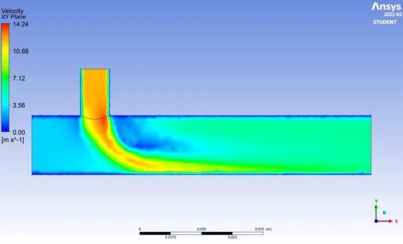
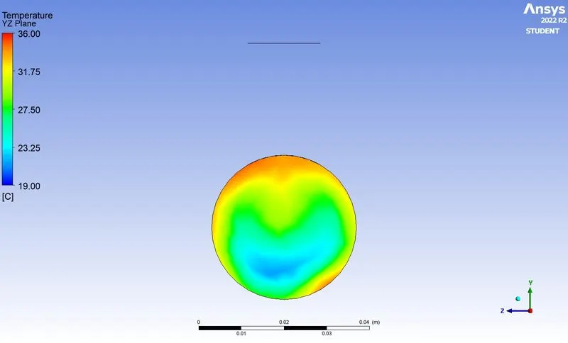
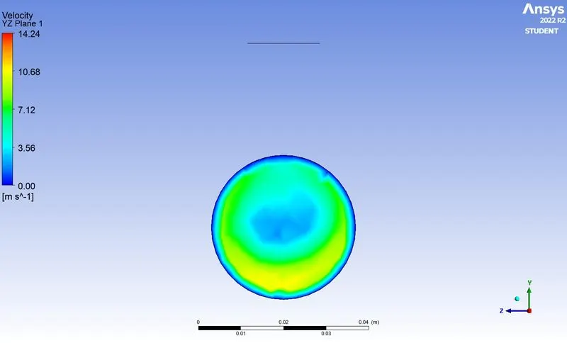
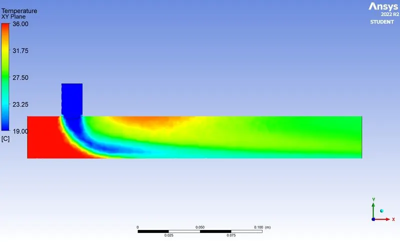
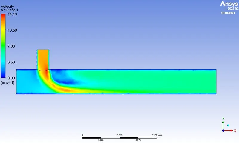
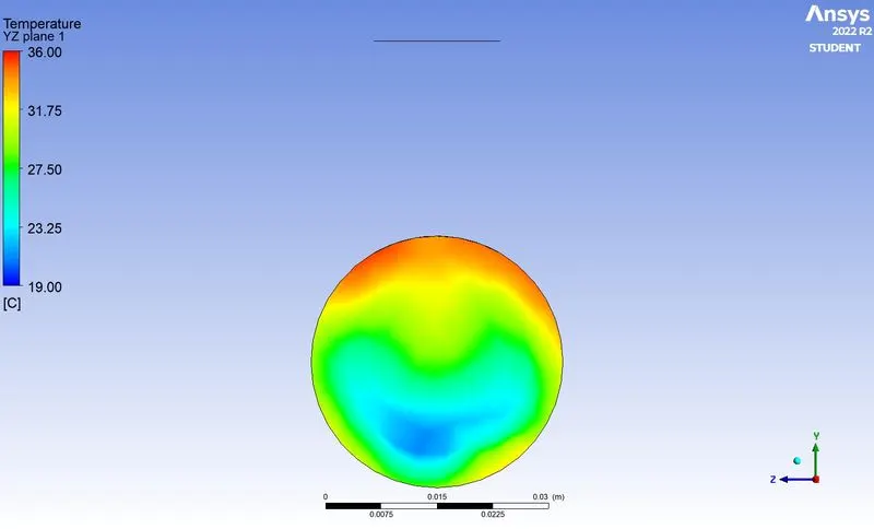
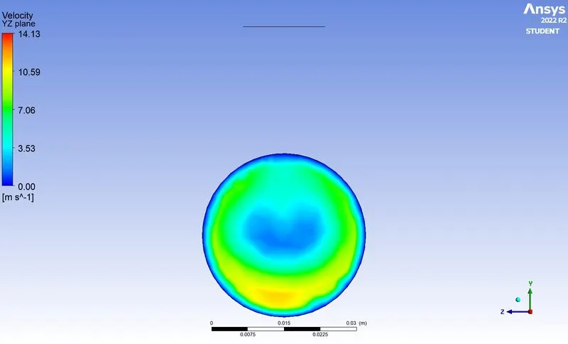
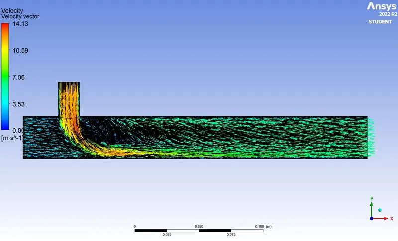
• Create a new XY plane and YZ plane to capture temperature and velocity contours along and across the model.
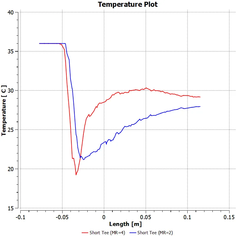
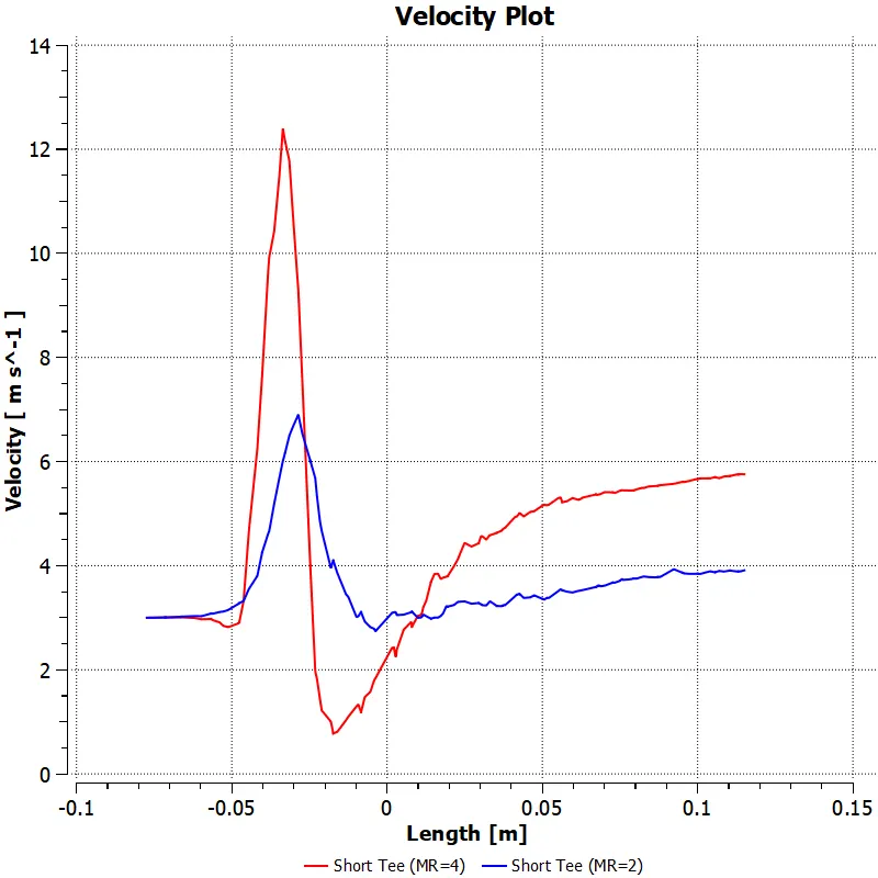
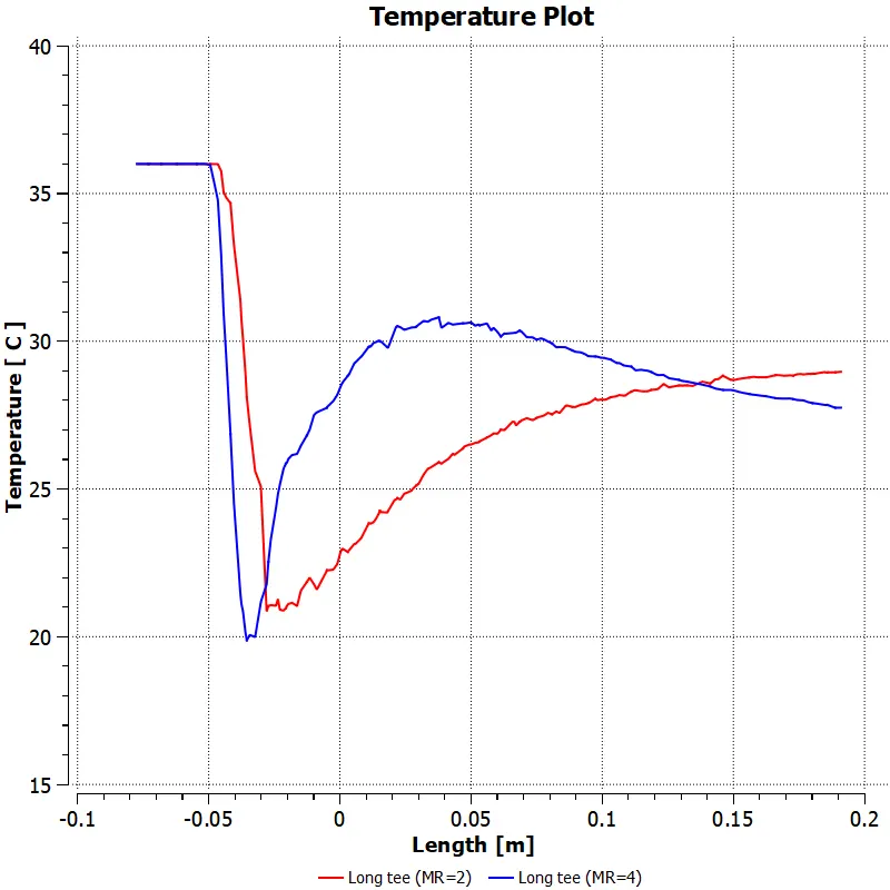
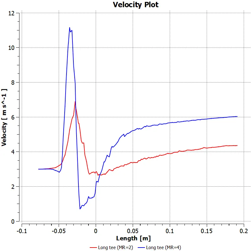
• Temperature and velocity variations can be obtained by creating a new line and using the chart tool.

Selection of Turbulence Model:-

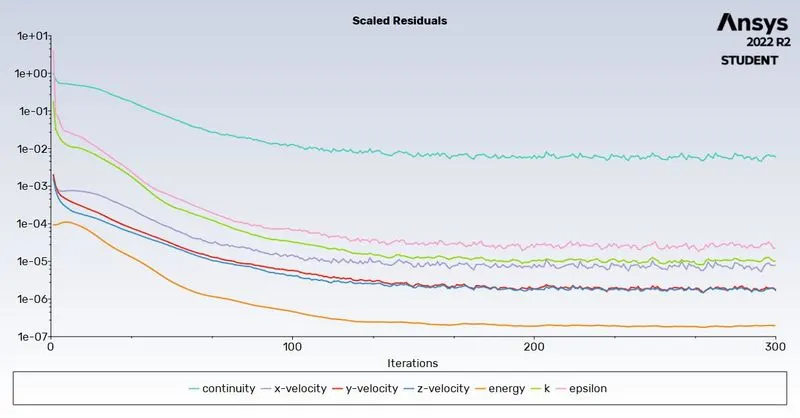
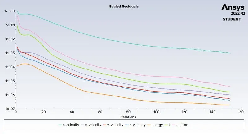
• in order to find the best-suited turbulence model, we will run the first case using both the k-epsilon and k-omega SST models.

k-epsilon model

k-omega SST model

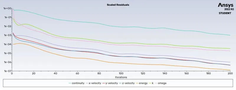
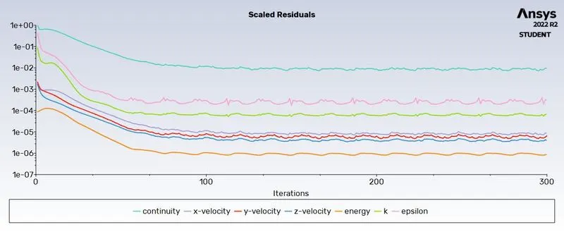
• From the above residual plots, we can see that the k-omega SST model is taking more time compared to the k-epsilon model for achieving convergence criteria.
• So for further cases, we will use the k-epsilon model as it will take less time compared to the other model.

Results:-

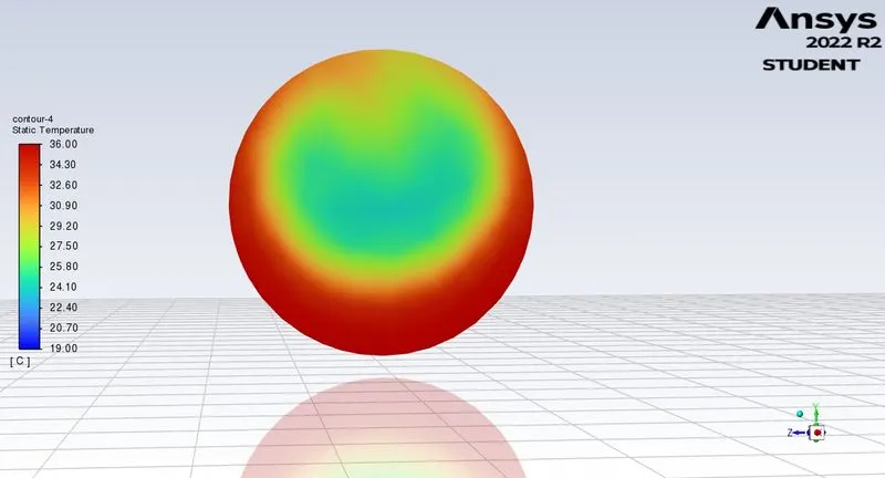
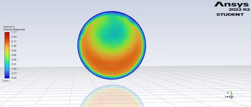
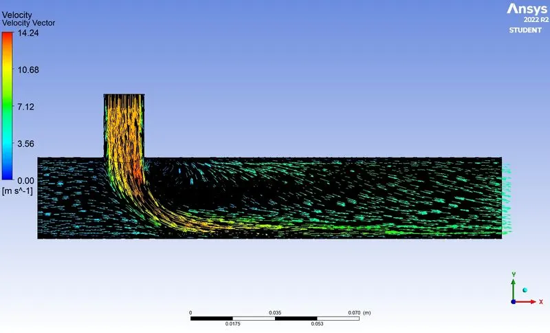
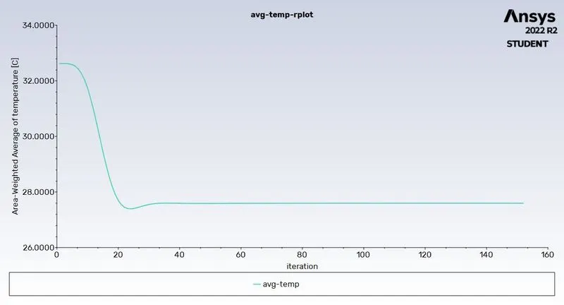
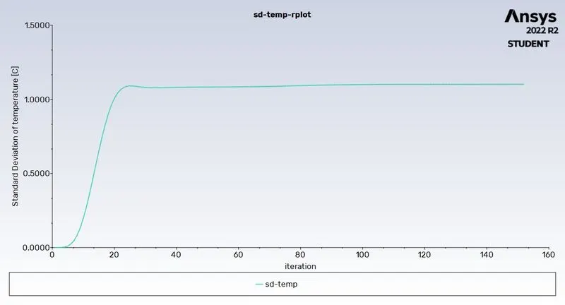
After running all the cases, we can now look at the results obtained.

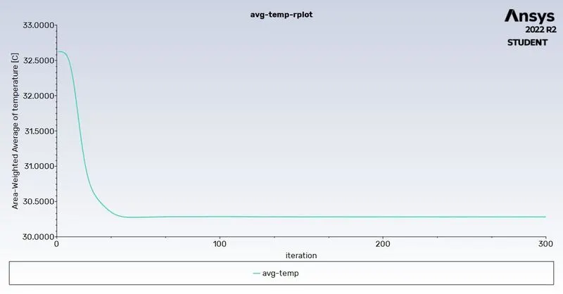
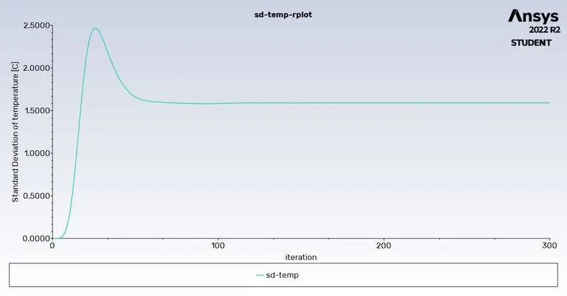
• Case 1a (Momentum ratio = 2)

• Case 1b (Momentum ratio = 4)

• Case 2a (Momentum ratio = 2)

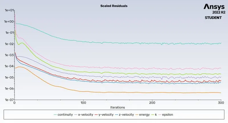
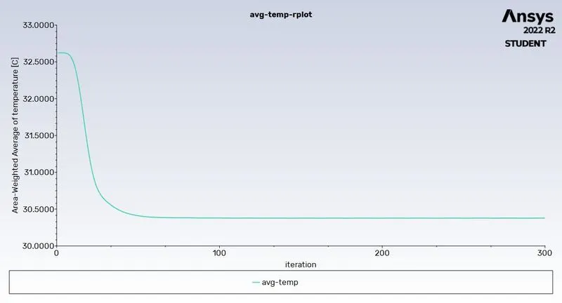
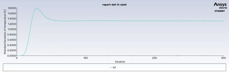
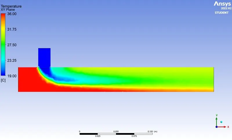
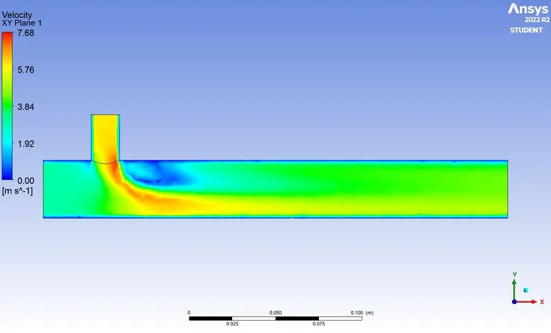
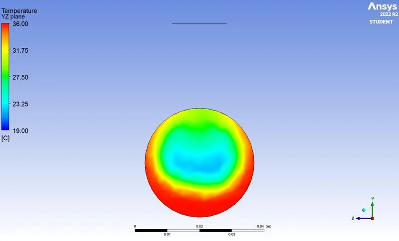
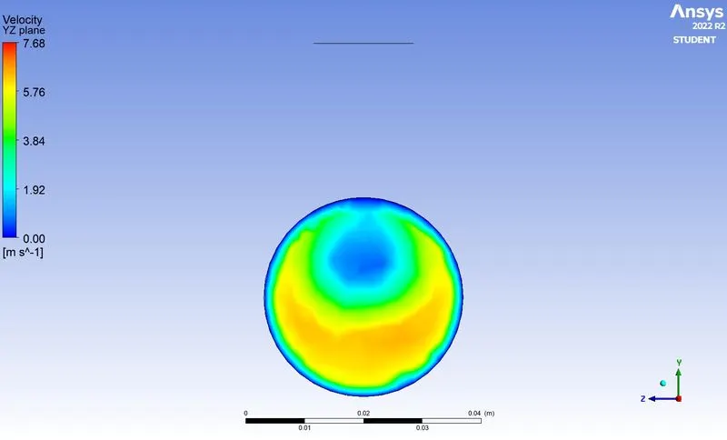
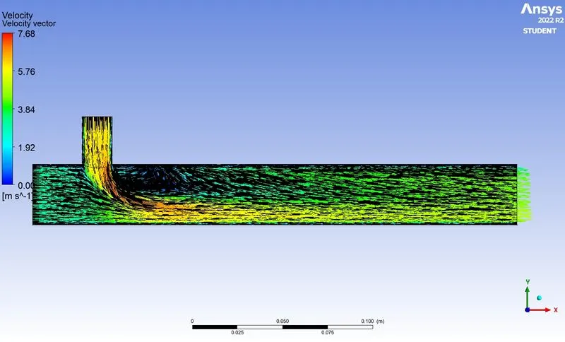
• Case 2b (Momentum ratio = 4)

	MR	Cell count	Avg outlet temperature (C)	Number of iterations for convergence
Case 1a	2	40039	30.277	200
Case 2b	4	40039	27.552	210
Case 2a	2	56878	30.377	150
Case 2b	4	56878	27.528	100

Conclusions:-

1. The outlet temperature is independent of the length of the mixing tee. In both cases, the temperature at the outlet is found to be similar
2. The momentum ratio affects the outlet temperature. By increasing the momentum ratio, the cold water inlet temperature increases which result in a drop in outlet temperature.
3. As wall effects are negligible and to save computational time, we used the k-epsilon model for our analysis.
4. By comparing the standard deviation of the outlet temperature of short and long mixing tee of momentum ratio of 4, it was observed that there was less deviation in the long one. So it is recommended to use the long mixing tee for effective mixing.
5. The value of average outlet temperature determined from the numerical simulation is found to be close the analytical value.