Week 1- Mixing Tee

Aim: To use Ansys-Fluent and run simulation for the given mixing tee geometry under specified conditions.

Objective:

We have two mixing tee geometries of different lengths. We pass hot air at 39⁰C and cold air at 19⁰C through the two inlets at different momentum ratios and study the mixing effectiveness and outlet temperature. We use and draw a contrast between k-epsilon and k-omega SST turbulence models and conduct the simulation with the best turbulence model.

Introduction:

Mixing tees are predominantly used in petrochemical industry to reduce thermal fatigue of the pipelines, blending oils and in waste water treatment plants. This also has application in air-conditioning systems. The geometry consists of an arrangement using which we can achieve good amount of mixing of the input fluids as shown in the following figure.

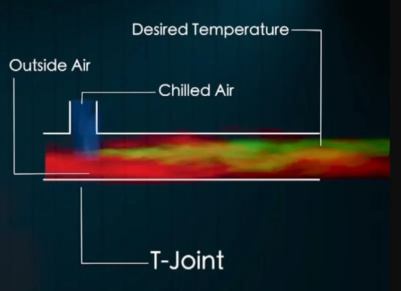
The mixing effectiveness can be varied by altering the angle of the branch pipe which changes the way the two fluids interact. The fluid entering from the branch pipe causes sudden turbulence at the interaction point causing large turbulent eddies which cause efficient mixing of the two fluids as they move downstream along the pipe.

Theory:

Experiments performed to study the physics of certain phenomenon is costly and time-consuming. Numerical simulation is developed and used to reduce the time needed to study the nature and physics of the system of interest. This method indeed provides results very fast compared to experiments but they lack a bit in terms of accuracy. If the experiments take a month to produce results, simulation might take a day and give us results 90% accurate. In the fast-paced world, where developing various solutions require faster results, engineers make a delicate balance between the accuracy and time taken as necessary.

All fluid flows are governed by three equations -Continuity, momentum and energy equations. We need to solve these equations for the given conditions to understand the fluid behavior. Computers are incapable of solving these equations in their integral and differential forms. So, we can divide our geometry into many tiny elements (called mesh) and modify the governing equations into difference equations that can be solved by the computer. We apply these difference equations for all the elements in the geometry and generate an approximate solution. It is hence necessary to validate these results against the experimental data.

The number of difference equations, for a given problem varies with the nature of physics involved. We typically solve a finite number of equations at all the elements. These equations are grouped together, called a turbulence model. A lot of work has been put into developing and improving the turbulence models and the work still goes on today. Examples of turbulence models are S-A, k-epsilon, k-omega etc.

Analytical solution:

We use the continuity equation to calculate the outlet velocity and energy balance equation to calculate the outlet temperature for the specified input parameters.

Given data: For MR = 2 (velocity of cold air/ velocity of hot air)

Diameter of hot inlet (Dh) = 0.0339 m

Diameter of cold inlet (Dc) = 0.017 m

Temperature of hot inlet (Th) = 39 ⁰C

Temperature of cold inlet (Tc) = 19 ⁰C

Velocity of hot air (vh) = 3 m/s

Velocity of cold air (vc) = 6 m/s

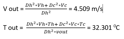
We similarly get results for other cases as tabulated.

Model	Momentum ratio	Outlet temperature (0C)	Outlet velocity (m/s)
For both short tee and long tee	MR = 2	32.301	4.509
	MR = 4	28.967	6.018

Modelling Approach:

The work flow in Ansys Fluent would follow four steps:

1. Geometry creation.
2. Mesh generation.
3. Pre-processing settings and simulation.
4. Extracting results.

Geometry creation:

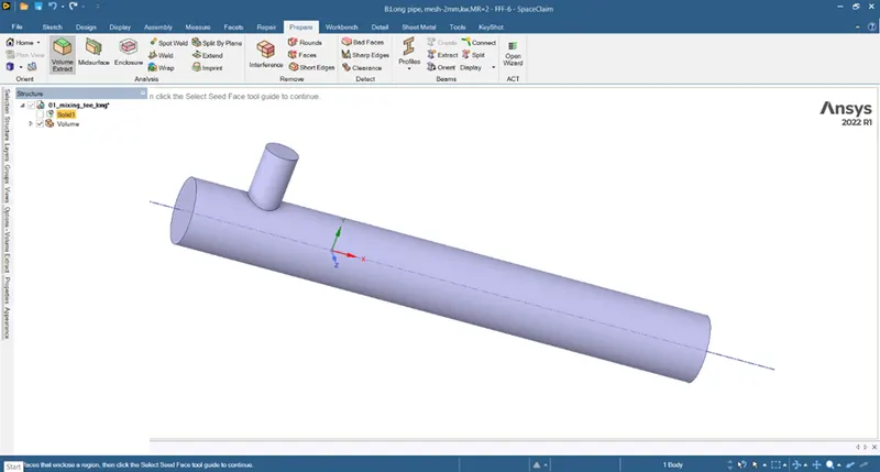
We drag and drop the Fluent module to create the standalone system. We open the geometry editing section- Space claim.

We import the given geometry to Space claim and create the fluid volume using Prepare -> Volume Extract -> Select the edges. We can suppress the solid volume in the Structure section as we are interested only in the fluid behavior. We can close the window and the changes made in the geometry are updated to our standalone system.

Mesh generation:

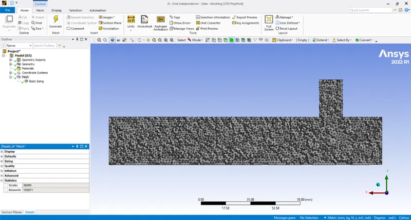
We will proceed with mesh generation for required mesh element length using the Sizing and Inflation options. We use Mesh -> Insert -> Sizing, to specify the size of the mesh elements in the given volume. We use Mesh -> Insert -> Inflation, to create inflation layers near the specified boundary.

We assign appropriate named selections to make it easier to work in the simulation section later. Here, we assigned the flow inlets, outlet and wall. We close the window and the changes are updated in the system.

Pre-processing settings and Simulation:

We would proceed to Setup the conditions of the model. The process flow would be as follows:

1. Check the mesh in the solver.
2. Modify units of Temperature to Celsius.
3. Choose the turbulence model and enable energy equation.
4. Specify boundary conditions.
5. Create necessary surface plots that we need to investigate.
6. We initialize and run the simulation for given number of iterations.

Extracting results:

We open the results section where we can use various visualizing tools like transparency and colouring the created surfaces with the instantaneous variables like temperature, velocity and obtain contours and plots.

Settings used for current simulation:

We used Pressure-based solver, absolute velocity formulation, steady state simulation and also solved energy equation.

We used k-epsilon and k-omega turbulence models. We used air as working fluid with default properties.

Grid Dependency test:

We have to ensure that the solution does not depend on the number of elements in the model. So, we run few simulations with different number of mesh elements. This is called Grid dependency test, where we decide the minimum number of elements required to make sure the solution is acceptable.

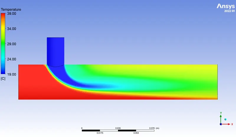
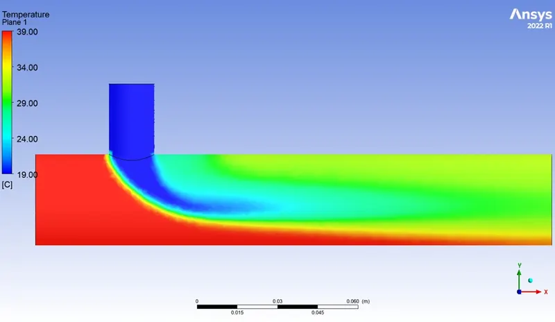
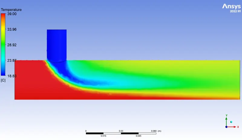
For the given geometry, we would run grid dependency test for four cases: 1mm, 2mm, 3mm and 5mm. We have used the following parameters for grid dependency test.

Mesh Length	1mm	2mm	3mm	5mm
No. of elements	15,37,152	1,93,053	74,490	20,103

We have run the simulation for he above mentioned pre-processing settings and have drawn a contrast for the temperature contour extracted in XY plane at the center of the geometry.

For 1mm:

For 2mm:

For 3mm:

For 5mm:

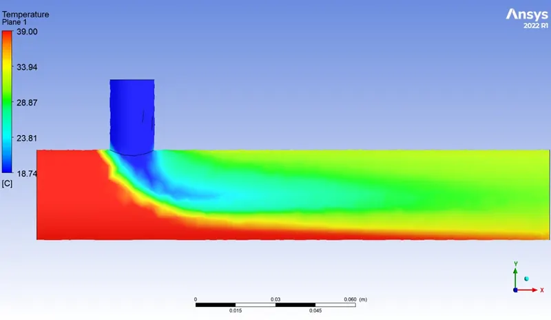
The results in 3mm and 5mm mesh seem distorted near the fluid interaction zone. This can be attributed to the coarse mesh elements at the interface. The value of the variable at the centroid of the mesh element decides the colour of the element. The results for 1mm and 2mm look almost the same, while the latter has little disturbance at the fluid interface, it is within the allowable range.

Hence, we can proceed with 2mm mesh elements for the rest of our study.

Comparison between k-omega and k-epsilon models:

We were asked in the problem statement to run simulations for two turbulence models: k-epsilon and k-omega. We will choose the same geometry and conditions as used in earlier study and proceed with k-omega model. We observe a little difference in the results given by the two models as shown in the following two figures.

Temperature contour for k-epsilon model:

Temperature contour for k-omega model:

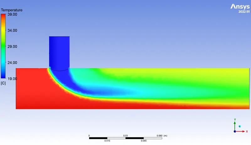
The mixing of fluids in k-epsilon model seems to be complete earlier than in the k-omega model. This result can be because epsilon equation captures dissipation of turbulent kinetic energy(k) and omega equation captures rate of change of epsilon. Hence k-omega can be considered superior based on this observation.

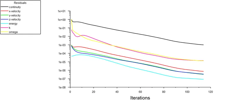
Also, for the given geometry and conditions k-omega model converged to the specified criteria earlier than k-epsilon model.

Model	No. of iterations
k-epsilon	237
k-omega	128

From the above-mentioned reasons, we conclude k-omega model is better and will be used for further study.

Short tee, MR=2:

The simulation used in the earlier k-omega simulation is for his configuration and we extract results.

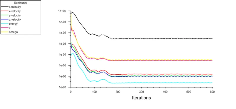
Scaled residuals:

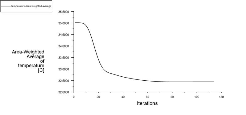
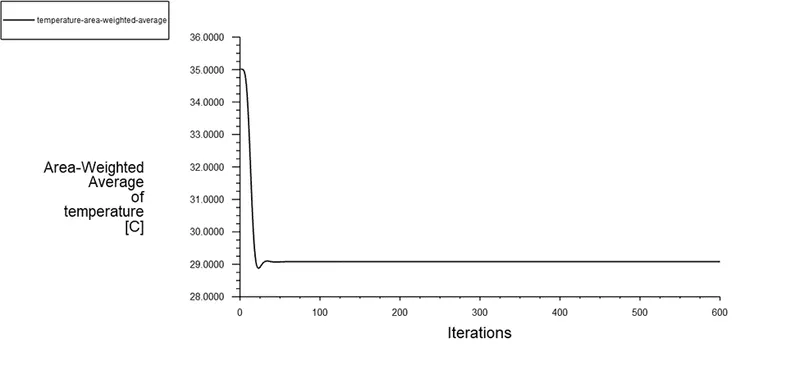
Area- weighted average of temperature at outlet:

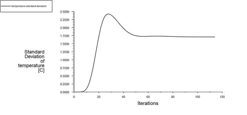
Standard deviation of temperature at outlet:

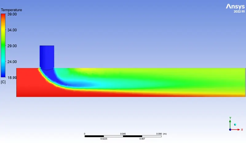
Temperature contour:

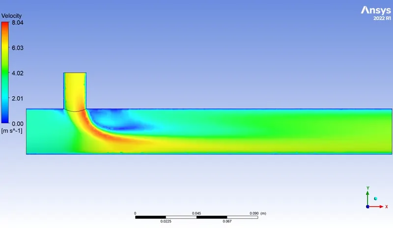
Velocity contour:

Short tee, MR=4:

The pre-processing settings would be same as in the previous case except we input the inlet velocity as 12 m/s. We have obtained the following results.

Area- weighted average of temperature at outlet:

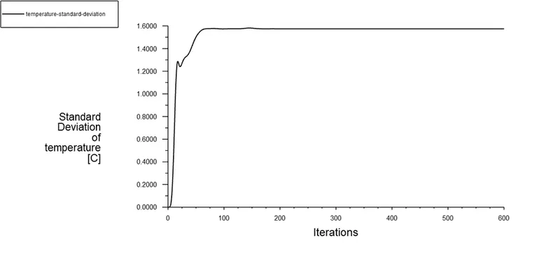
Standard deviation of temperature at outlet:

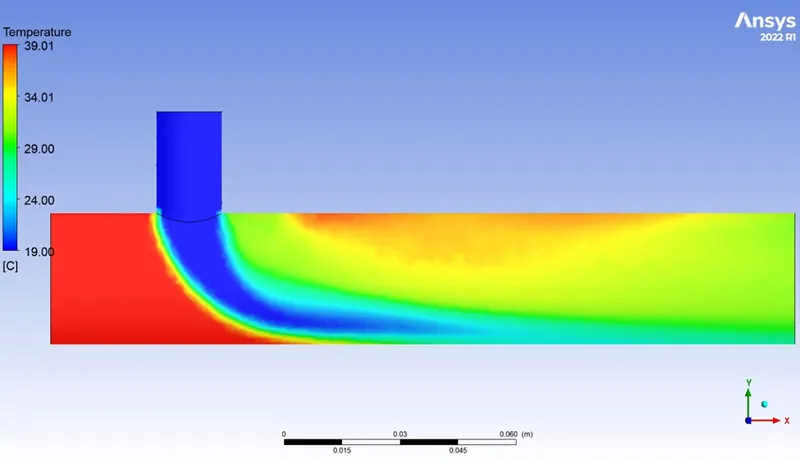
Temperature contour:

Velocity contour:

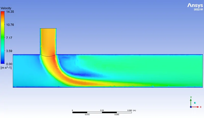
From the above observed results for the short tee model for different momentum ratios, we make the following observations.

	Inlet velocity (m/s)	Outlet temperature (0C)	Deviation in temperature (0C)	Outlet velocity (m/s)
MR = 2	6 m/s	32.418	2.529	4.505
MR = 4	12 m/s	29.081	1.574	6.064

Long tee, MR=2:

We create the geometry, perform mesh in the similar way we did it for the short tee configuration. We input the same pre-processing values used for the short tee MR=2 and run the simulation. We have obtained the following results.

Scaled residuals:

Area- weighted average of temperature at outlet:

Standard deviation of temperature at outlet:

Temperature contour:

Velocity contour:

Long tee, MR=4:

The pre-processing settings would be same as in the previous case except we input the inlet velocity as 12 m/s. We have obtained the following results.

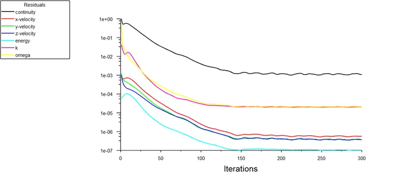
Scaled residuals:

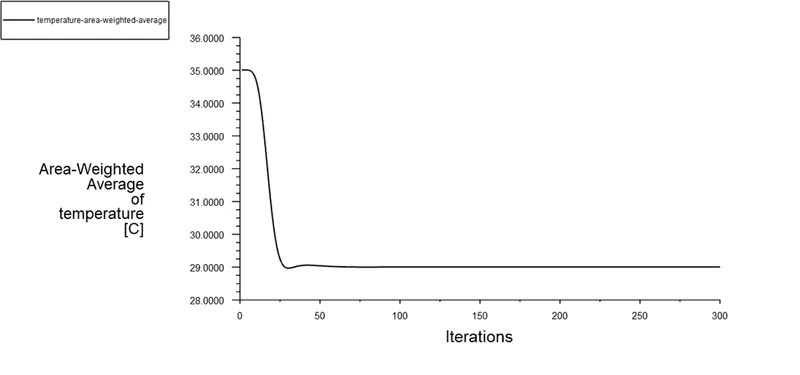
Area- weighted average of temperature at outlet:

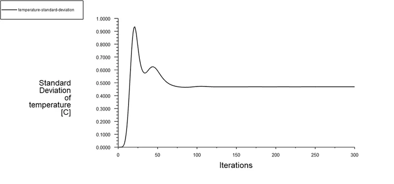
Standard deviation of temperature at outlet:

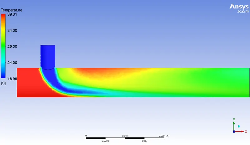
Temperature contour:

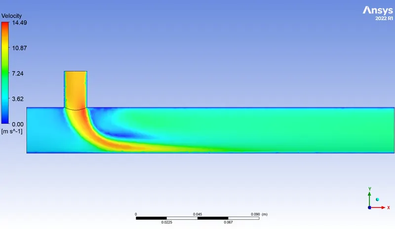
Velocity contour:

From the above observed results for the short tee model for different momentum ratios, we make the following observations.

	Inlet velocity (m/s)	Outlet temperature (0C)	Deviation in temperature (0C)	Outlet velocity (m/s)
MR = 2	6 m/s	32.442	1.71	4.498
MR = 4	12 m/s	29.004	0.469	6.021

Results:

Validation of results:

We can calculate the deviation in the results of velocity and temperature obtained from the simulation with the analytical solution calculated earlier. The details are tabulated.

Model	Momentum ratio	Error in Outlet temperature (0C)	Error in Outlet velocity (m/s)
Short Tee	MR = 2	0.36	0.09
	MR = 4	0.41	0.76
Long Tee	MR = 2	0.44	0.05
	MR = 4	0.13	0.05

The deviations are very small and hence we can say the simulated results are accurate.

Conclusion:

We observe there is less temperature for given configuration MR=4 because of more mass flow rate of cold air and hence more cooling.

We also observe the standard deviation at outlet for long tee for given MR is less than short tee since more mixing occurred due to increased length.

References:

1. https://www.hydrocarbonprocessing.com/magazine/2020/august-2020/special-focus-valves-pumps-and-turbomachinery/cfd-modeling-of-mixing-tees-design-of-a-thermal-sleeve
2. https://core.ac.uk/download/pdf/242403155.pdf
3. https://www.sciencedirect.com/science/article/abs/pii/S0029549309005676