Week 1- Mixing Tee

Objective of this exercise is to simulate air flow through a mixing tee section and try to understand the effects of change in mixing effectiveness with change in the length of the section. We try to do the simulation for two versions of the section, one is longer and one is shorter.

A tee section or 'T' section is one which is used most widely in many applications where a proportionate mixing of particles or substances are required. Controlled mixing of the substances can be achieved by using this technique and some of the most common applications are in air conditioners, in industrial applucations such as radiators, and for fluid mixing as well. Good temperature control and homogeneous mixtures can be achived using this techniques. We use a model for short as well as long tee sections, define the parameters and specify boundary conditions in order to simulate and post process the results.

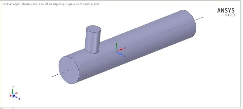
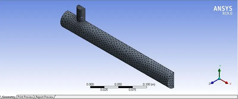
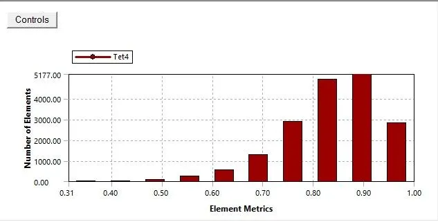
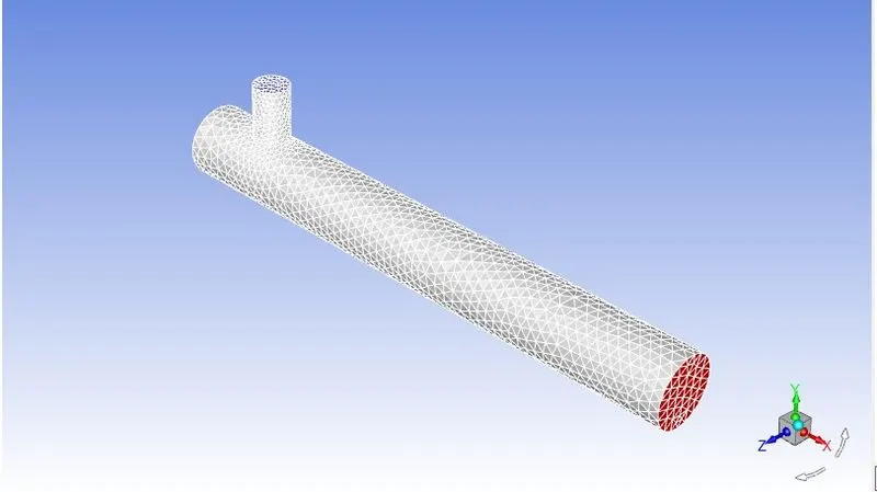
At first, a solid section of the above shown model, which is the smaller tee section is obtained from which only the flow volume is required for the purpose of simulation. Therefore, we neglect all the other sections and chose the flow volume, suppress the solid section from being called for the simulation and then save it inside the geometry part of the fluent in workbench. After that, we update the geometry, and enter into mesh, where we create named selections for the inlets, outlets, and the walls. Then, we can change the sizing of the mesh from coarse to fine, under the quality of mesh, change the mesh metric to element quality, and cut the part to obtain a section for detailed analysis of meshing process after the mesh has been generated.

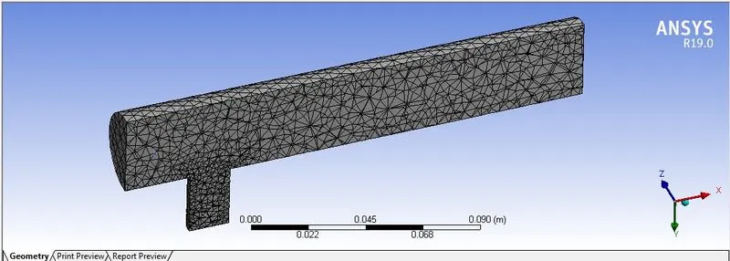
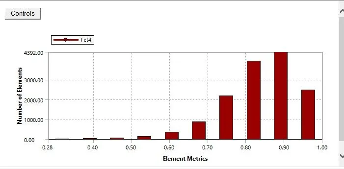
Now, we can select the setup option and get into the fluent, by selecting the double precision, then iside, we have to set up the domain first.

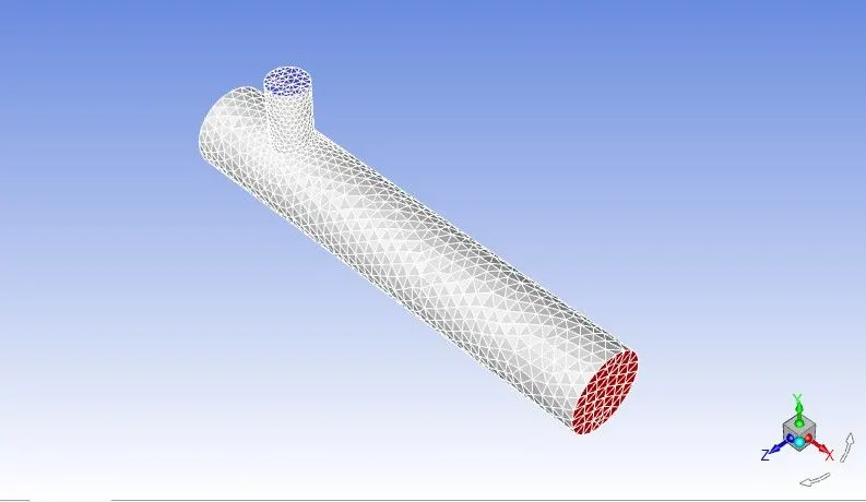
Here, we check the mesh quality, go into the console and check for any errors in the mesh. Then, under setting up physics, we use steady state, pressure based absolute conditions, and since we need the temperature values, we check the energy option. After specifying the parameters, we specify the type of material, which in our case is air. Then, under zones, cell-zones, we can again check for the volume-volume option and the material specified. Now, under boundaries, we specify the boundary condtions necessary for our simulation process. Under models, we select k-E model for the first simulation and use realizable for standard wall functions.

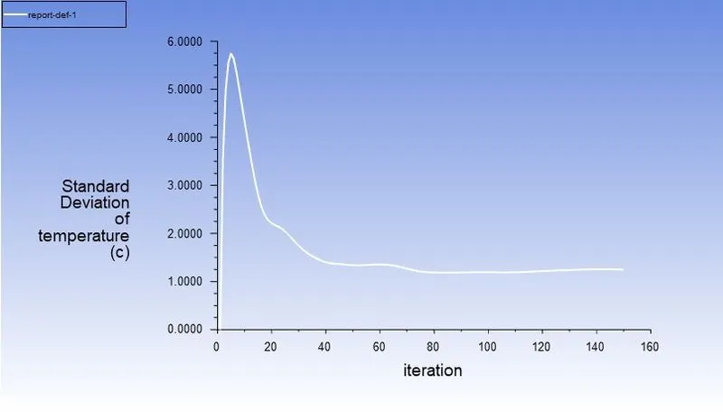
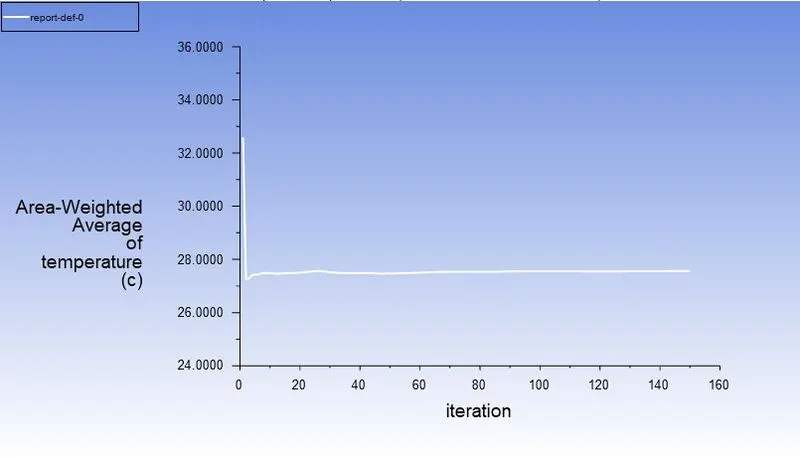
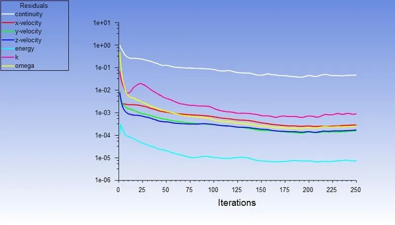
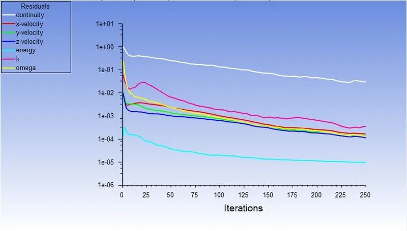
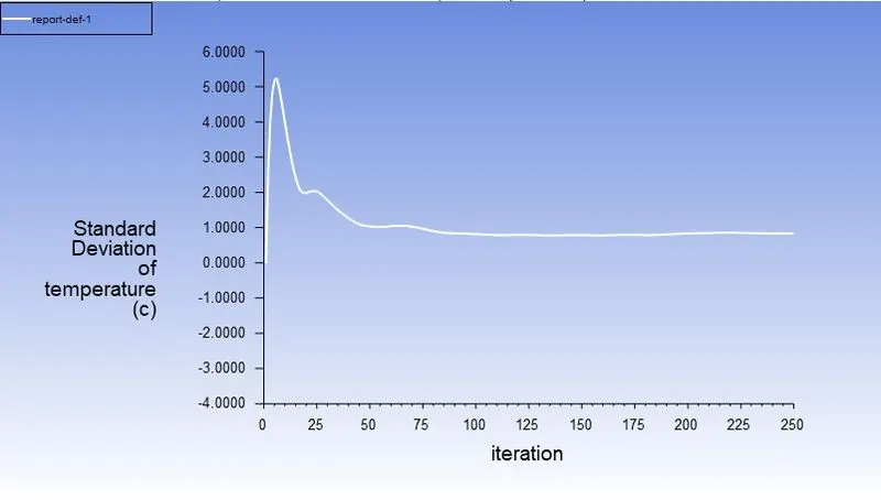
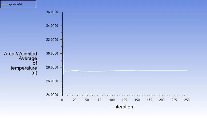
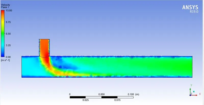
Under the boundaries, for our cold and hot inlets, we specify the temperatures and the velocities based on the corresponding momentum ratios provided. Then, we check for the outlet boundary conditions and then under solving option, we chose hybrid method and initialize the process. We specify the number of iterations, then run the calculation. The plots obtained are as follows:

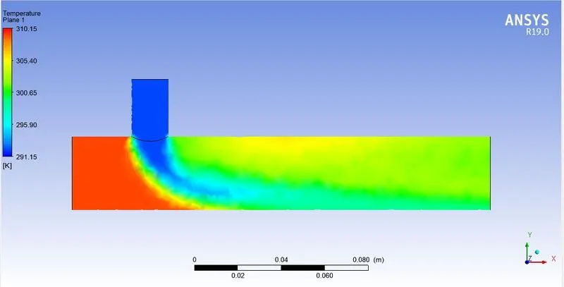
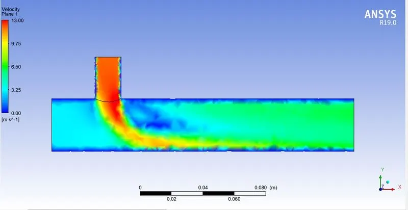
For k-`epsilon`model and momentum ratio of 2:

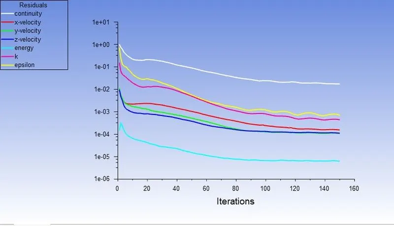
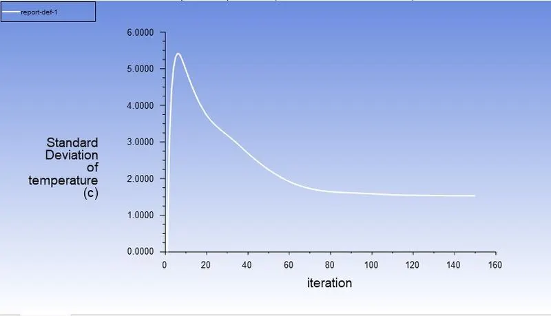
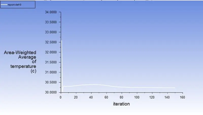
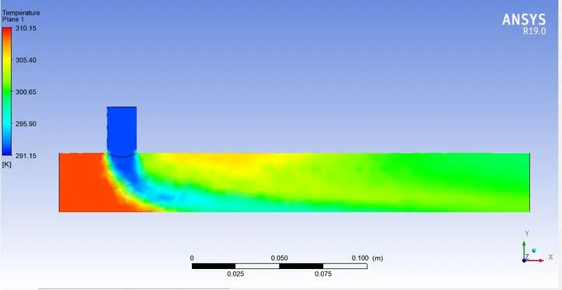
Now, under the results option, we select the sections, and we create an xy plane to slice the section, set up the variable as temperature, and range as user specified, for plane1 created, and specify the range.

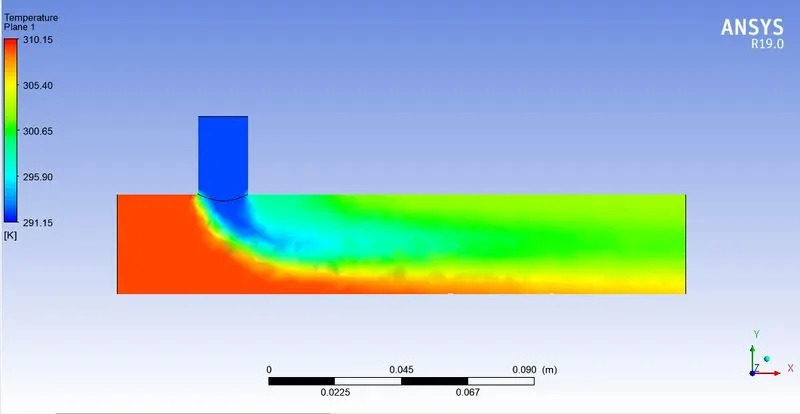
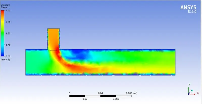
Now, this process is repeated for the same small tee section for change in momentum ratio and for k-omega sst model.

For k-`epsilon`model and momentum ratio = 4:

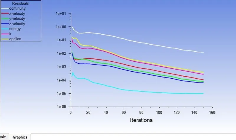
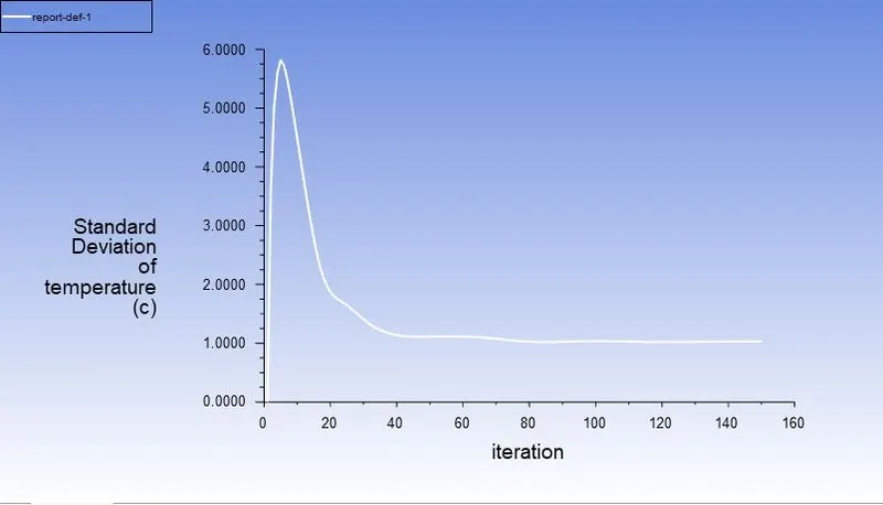
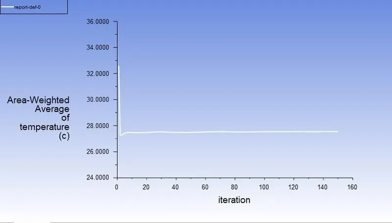
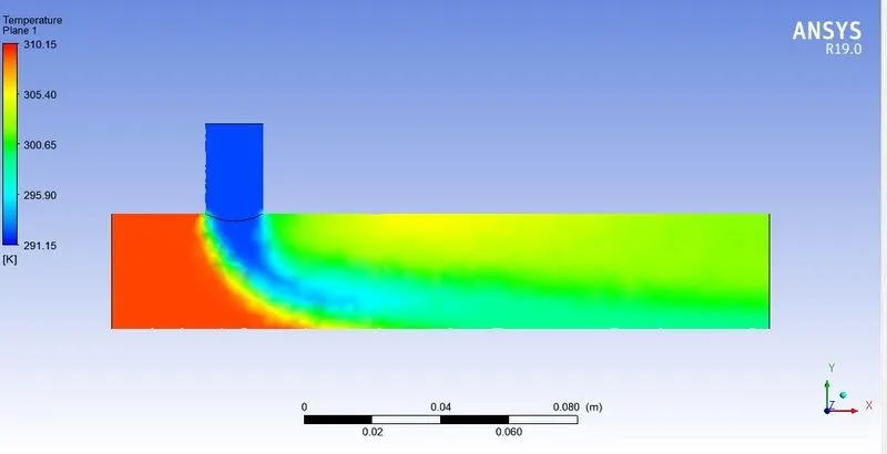
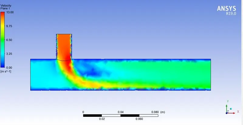
For k-`omega`model and momentum ratio = 2 :

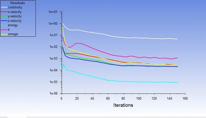
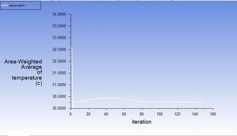
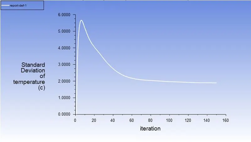
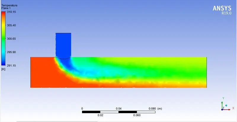
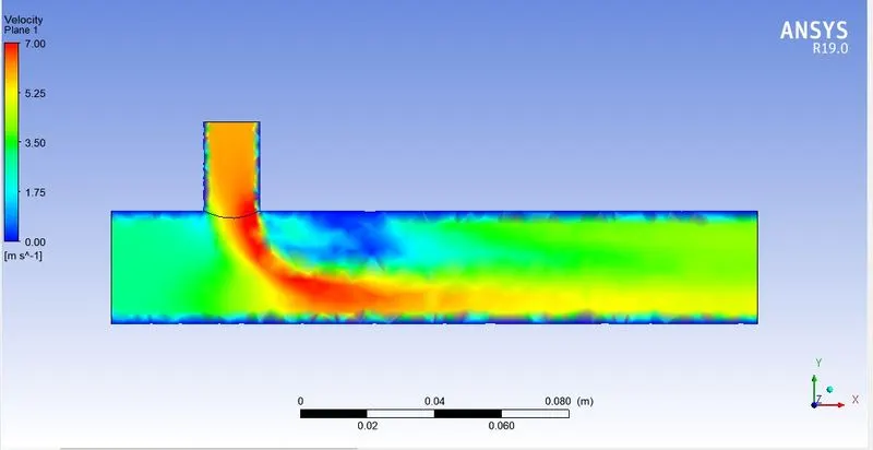
For k-`omega`model and momentum ratio = 4 :

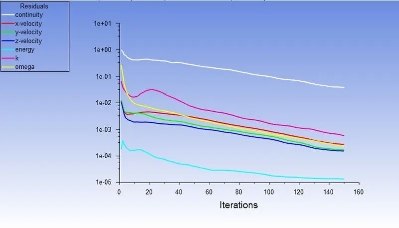
From the above simulations, we choose k-`omega`model for the long mixing tee section. This is primarily because for flows near the wall regions, k-`omega`models are the best suitable ones.

For k-`omega`model and momentum ratio = 2 (long mixing tee):

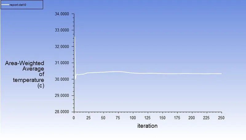
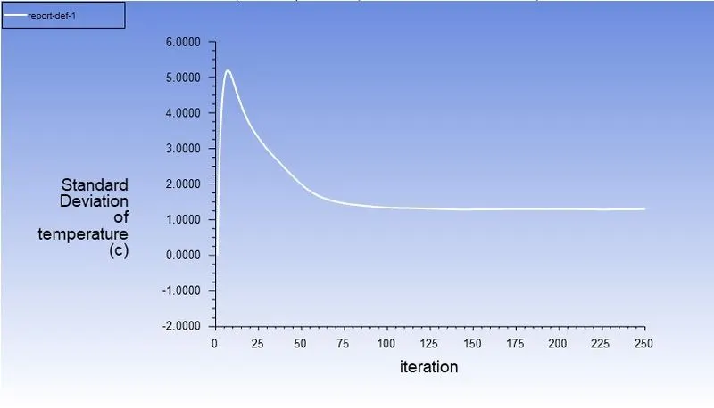
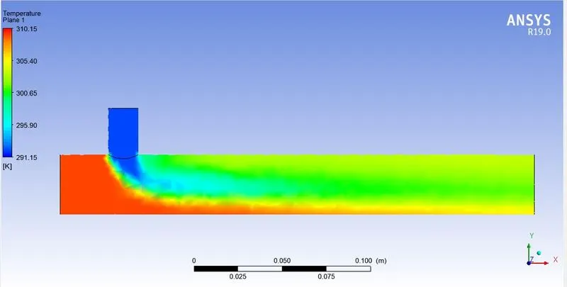
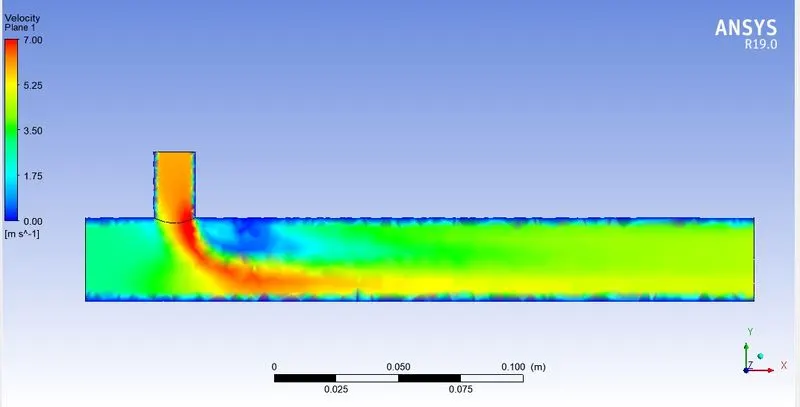
For k-`omega`model and momentum ratio = 4 (long mixing tee):

Type	Cell count	Outlet Temp (avg in Kelvin)	No. iterations for convergence
Short tee - ratio = 2 (k-`epsilon`)	14349	304.038	200
Short tee - ratio = 4 (k-`epsilon`)	14349	300.719	250
short tee - ratio = 2 (k-`omega`)	14349	304.145	200
short tee - ration = 4 (k-`omega`)	14349	300.635	250
long tee - ratio = 2 (k-`omega`)	17886	303.741	250
long tee - ration = 4 (k-`omega`)	17886	300.333	250

From the simulation performed and based on the above results, it is evident that during the process of mixing, when the velocity of the cold inlet is increased, it prompts to more efficient mixing of the hot and cold air, and due to the turbulence occuring, the resulting outlet temperature is significantly lower when compared to the case where the cold inlet velocity is less. In comparison between the long and the short tee's, the air temperature measured at the outlet for a given long tee section is significantly lower than that for a short tee section as proper mixing can be prompted due to the increase in length and turbulant nature involving due to the higher inlet velocity for cold air inflow (greater momentum ratio) whereas in short tee sections, proper mixing does not occur for momentum ratio of 2 where it can be clearly seen through the plots that for a given short tee section, only some region of the hot air and the cold air get mixed thoroughly. Also, for the simulations to reach convergence, the number of iterations play a vital role and the mesh size as well. When we increase the number of iterations from 150 to 200 or 250, the convergence occurs and when we reduce the mesh size, the number of iterations increase as well and the simulation time is much higher comparitively. But, much more accurate results can be obtained by refining the mesh size and increasing the number of iterations.