Week 1- Mixing Tee

• AIM:

The aim of the challenge is to simulate the different cases of Mixing tee with different momentum ratios for two different lengths and to find the average outlet temperature and mixing effectiveness of fluids.

• THEORY:

Mixing tee ustilizes a specifically engineered intergral geometry to efficiently mix two fluid streams into one combined stream.Mixing tee is ideal for microbore or anlytical gradient HPCL.These mixing tee is specifically designed for high-pressure applications.Mixing tee is widely used in petrochemical industries,in which two fluid streams with different physical or chemical properties mix together.When their is large temperature difference between the two streams,large thermal fluctuion can occur in the region where two streams meet if proper design steps are not taken.The thermal flucations in metal may lead to thermal fatigue of the pressure boundary piping.If through-wall cracking occurs,fluid may leak,possibly causing a fire or damage.It is therfore imperative to make sure that the temperature flacuations are such the piping system can withstand them.Options may include improving the mixing of two streams to reduce the temperature flucations through redesigning of piping system such that the momentum ratio of the two fluid streams is favorable to rapid mixing or to install devices that protects the pressure boundary piping e.g injection quills or thermal sleeves in the region where the temperature flacutions are higher than the thermal fatigue threshold.

Computational fluid dynamics (CFD) modelling, such as well-resolved large eddy simulation (LES), can provide accurate predictions of the mixing behaviour, including velocity, concentration and temperature fields, in a mixing tee. The variations of the transient fluid temperature can therefore be used to identify a location in the main pipeline, after which the maximum temperature difference is less than a given value.

• TURBULENCE MODELS:

Turbulence modelling is the construction and use of a mathematical model to predict the effects of turbulence. Turbulent flows are commonplace in most real-life scenarios, including the flow of blood through the cardiovascular system, the airflow over an aircraft wing, the re-entry of space vehicles, among others. In spite of decades of research, there is no analytical theory to predict the evolution of these turbulent flows. The equations governing turbulent flows can only be solved directly for simple cases of flow. For most real-life turbulent flows, CFD simulations use turbulent models to predict the evolution of turbulence. These turbulence models are simplified constitutive equations that predict the statistical evolution of turbulent flows

K-epsilon model:

K-epsilon (k-`epsilon`) turbulence model is the most common model used in computational fluid dynamics (CFD) to simulate mean flow characteristics for turbulent flow conditions. It is a two-equation model which gives a general description of turbulence by means of two transport equations (PDEs). The original impetus for the K-epsilon model was to improve the mixing-length model, as well as to find an alternative to algebraically prescribing turbulent length scales in moderate to high complexity flows.

K-omega model:

In computational fluid dynamics, the k–omega (k–`omega`) turbulence model is a common two-equation turbulence model that is used as a closure for the Reynolds-averaged Navier–Stokes equations (RANS equations). The model attempts to predict turbulence by two partial differential equations for two variables, k and `omega`, with the first variable being the turbulence kinetic energy (k) while the second (`omega`) is the specific rate of dissipation (of the turbulence kinetic energy k into internal thermal energy).

• PROBLEM STATEMENT:

Compare the mixing effectiveness when hot inlet temperature is 36⁰C & the Cold inlet is at 19⁰C.

Use the k-epsilon and k-omega SST model for the first case and based on your judgment use the more suitable model for further cases. Giving the reason for choosing a suitable model is compulsory.

1. Case 1
   • Short mixing tee with a hot inlet velocity of 3m/s.
   • Momentum ratio of 2, 4.
2. Case 2
   • Long mixing tee with a hot inlet velocity of 3m/s.
   • Momentum ratio of 2, 4.

Momentum ratio = velocity at cold inlet / velocity at hot inlet

In a table, compare the following values from the 2 cases.

1. Cell count
2. Average outlet temperature
3. Number of iterations for convergence

CASE 1(A): SHORT MIXING TEE FOR M=2 (K-EPSILON MODEL)

• PROCEDURE:

1.The first step would be import the model into ANSYS spaceclaim for geometry clean-up

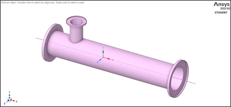
After importing we have to extract the volume which is in contact with fluid by using volume extract option and select the edges and then supress the geometry for physics

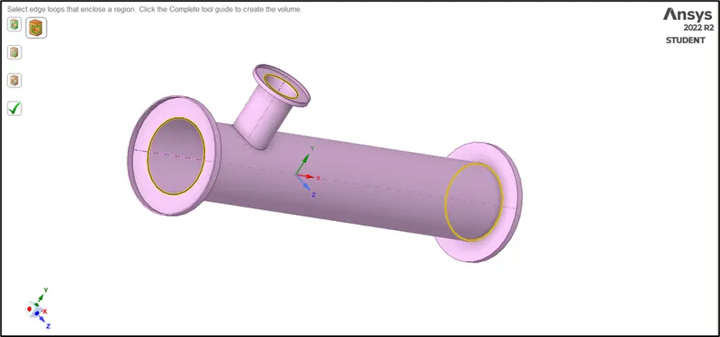
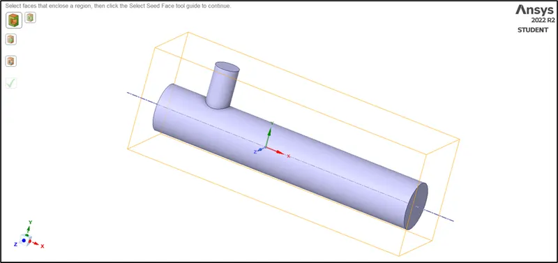
2. After preparing the model in ANSYS spaceclaim the next step would be meshing the model and before that we have to name the boundary by selecting the faces of the geometry

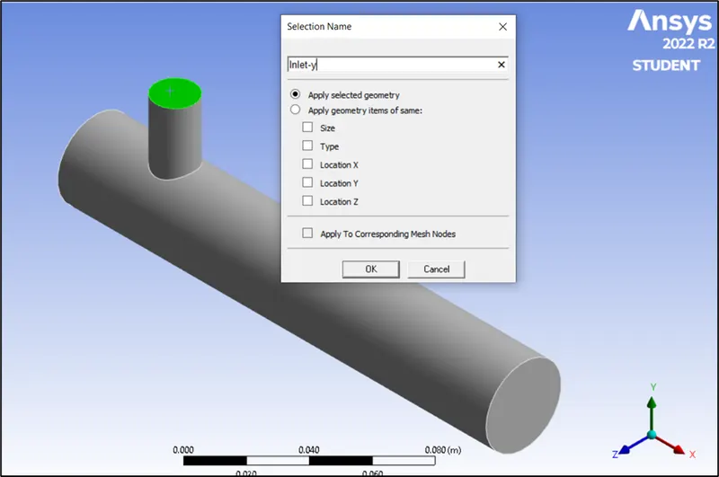
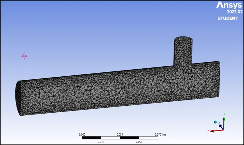
After naming the boundary we have to mesh the geometry with appropriate mesh size for study we using a element size of (2mm)

MESH: (ELEMENT SIZE =2MM)

ELEMENT QUALITY:

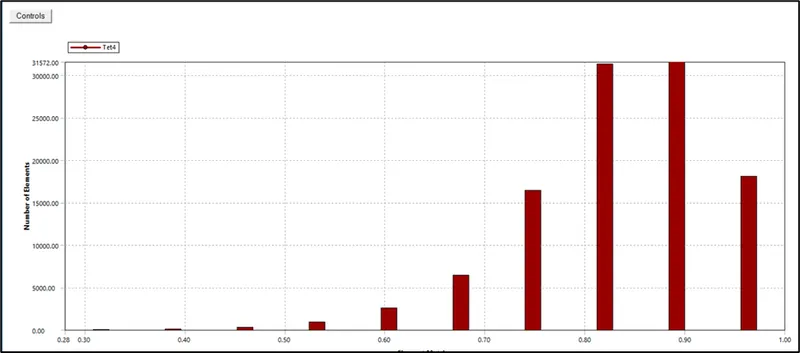
Most of the element quality is more the 5% so we can move ahead with this quality of mesh for our further studies.

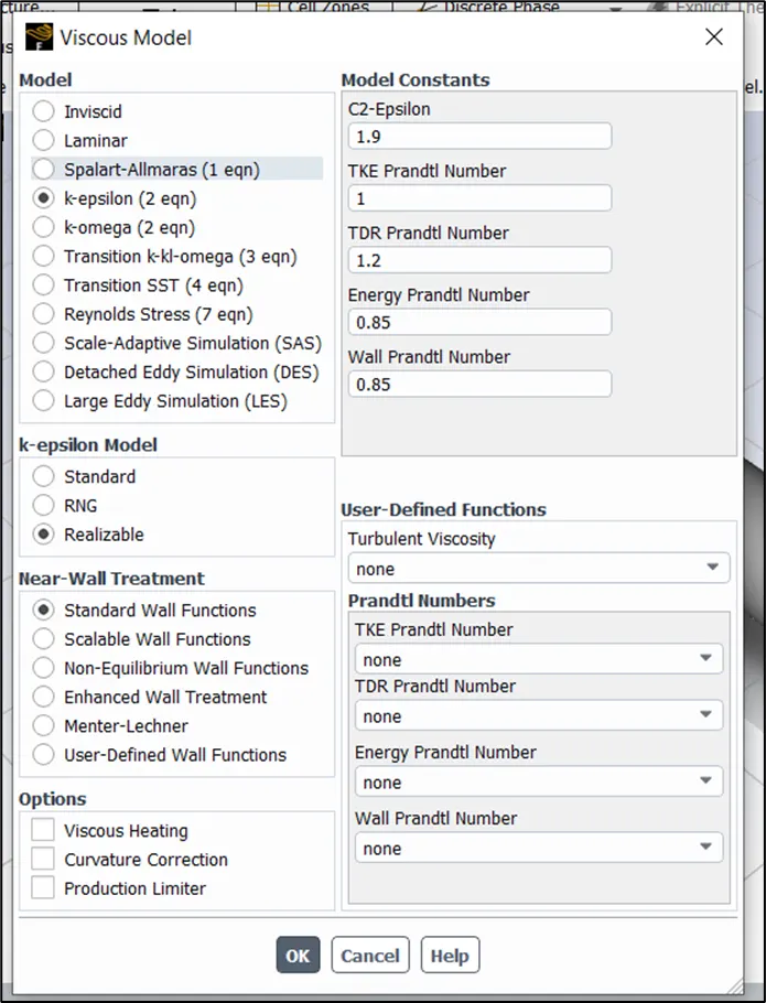
3.The next step would be set up the physics by enable the Energy for temperature calculation and for study we are using k-epsilon turbulence model with standard wall function near the wall under viscous model

SOLVER TYPE : PRESSURE BASED SOLVER

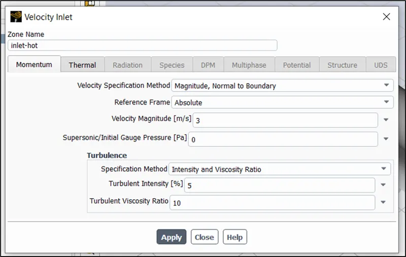
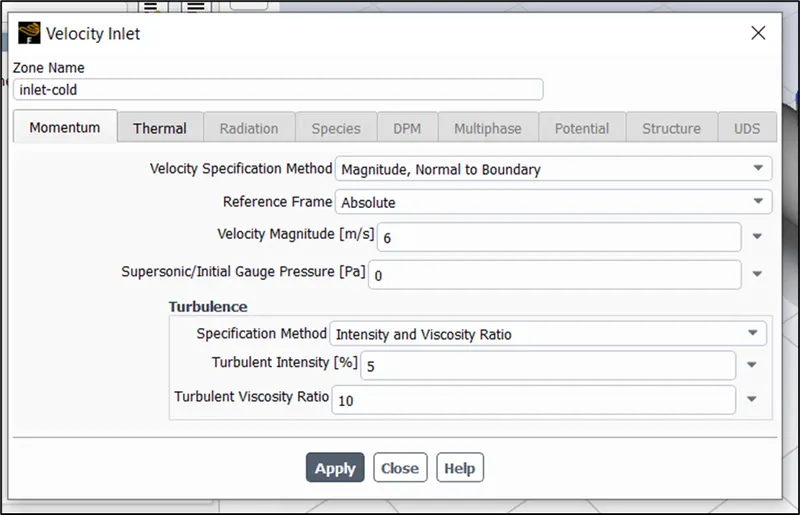
we are using following inputs

Velocity of hot air at inlet=3 m/s

Temperature of hot air at inlet=36 (C)

Momentum ratio = 2

Momentum ratio= velocity of cold inlet/velocity of hot inlet

velocity of cold inlet = 6 m/s

Temperature of COLD air at inlet=19(C)

4.SOLUTION INTIALIZATION:

The Solution Initialization allows you to set initial values for the flow variables and initialize the solution using these values.For study we are using the hybrid initialization .Hybrid initialization solves a number of iterations (10) of a simplified equation system and thereby gets usually a better guess for the flow variables, in particular for the pressure field.

After intialization we have to run the simulation for certain number of iteration untill solution gets converged.

• OUTPUT:

RESIDUAL PLOT:

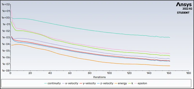
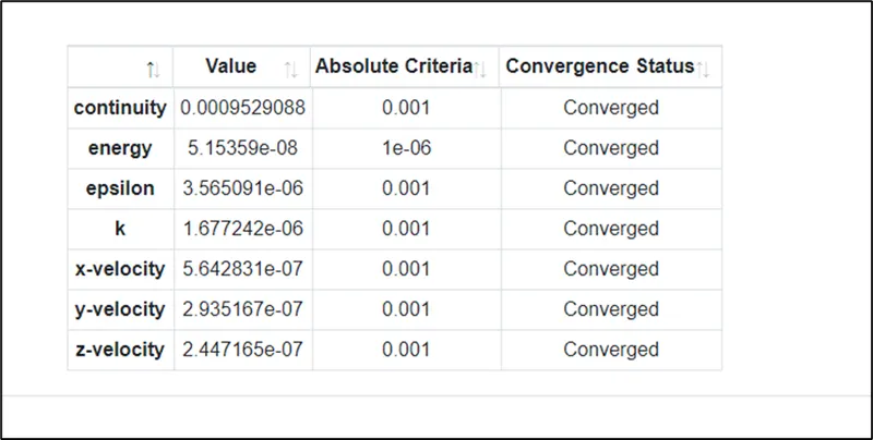
The solution is converged at 161 number of itteration

CONVERGENCE STATUS:

CONVERGENCE PLOT:

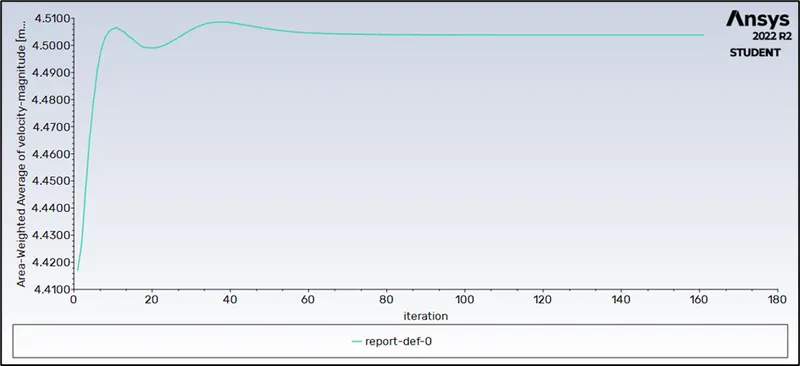
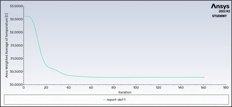
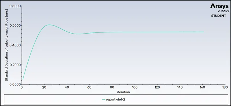
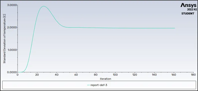
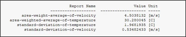
From the above observation average temperature and velocity at outlet is 30.28 C and 4.50 m/s

Temperature distribution:

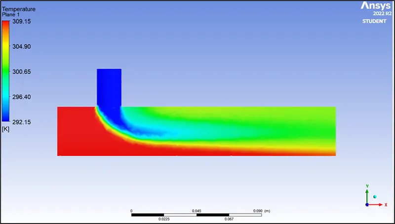
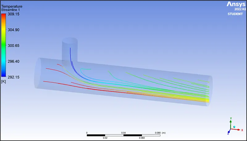
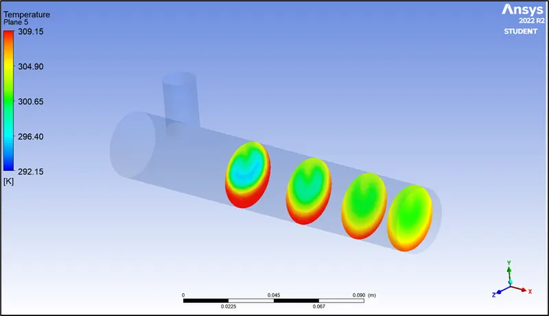
Temperature distribution across the plane:

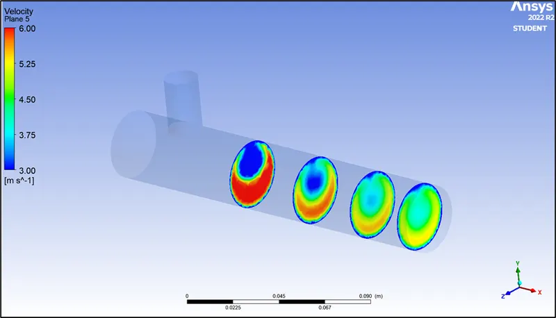
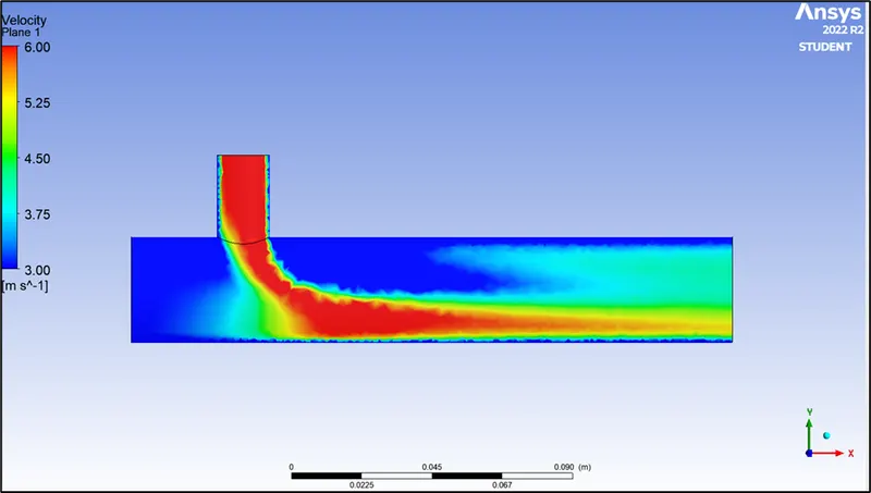
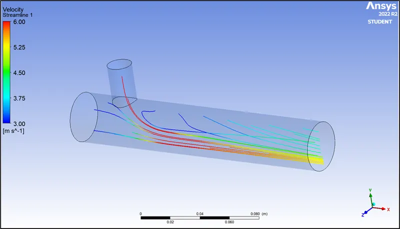
Velocity distribution:

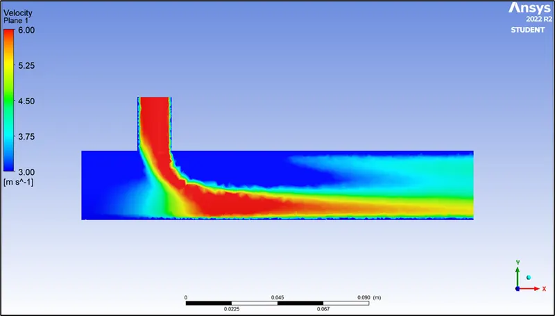
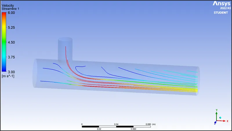
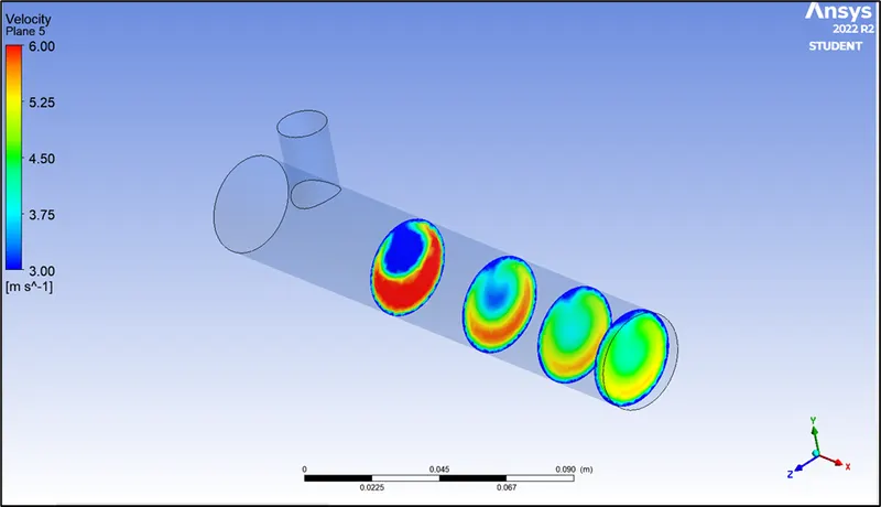
Velocity distribution across the plane:

FOR K-OMEGA MODEL:

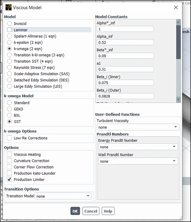
We are using k-omega SST turbulence model to capture the turbulence and remaining step are same as explained above

Viscous model:

• OUTPUT:

RESIDUAL PLOT:

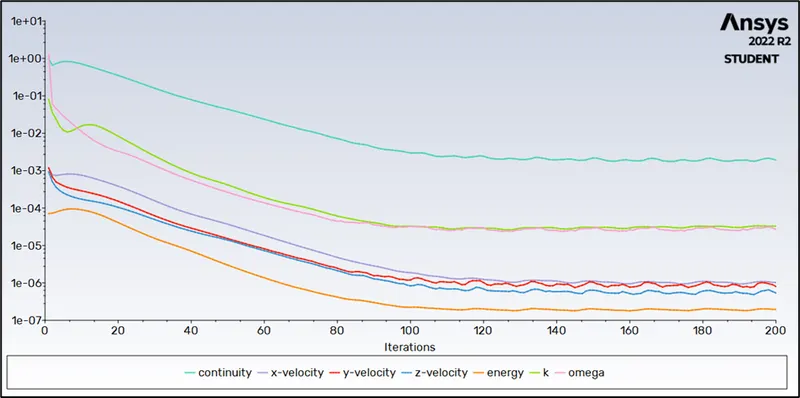
CONVERGENCE STATUS:

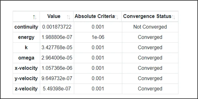
From above table we can see that mass is not conserved

CONVERGENCE PLOTS:

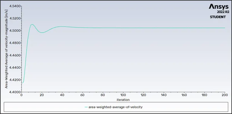
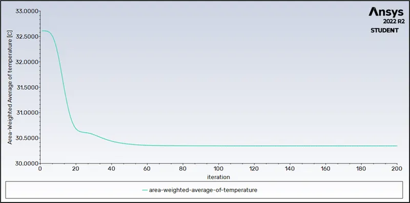
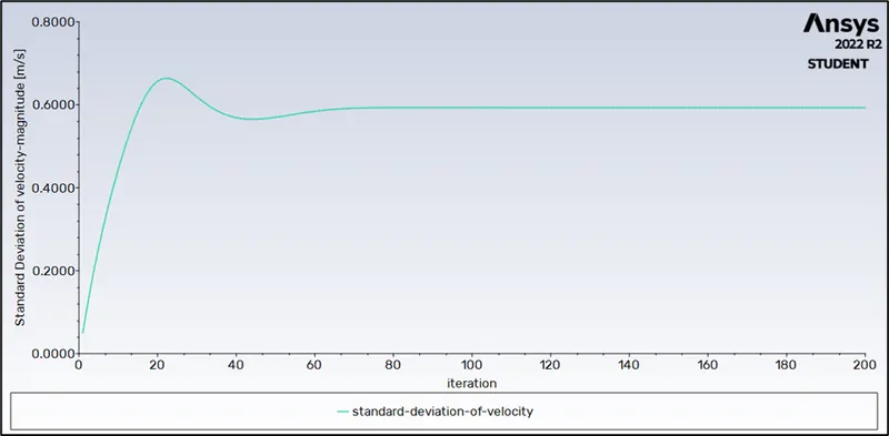
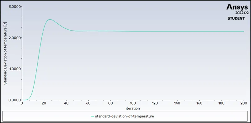
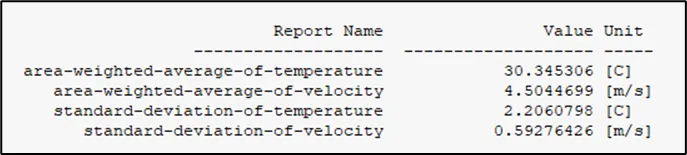
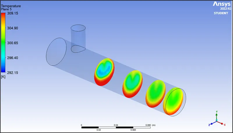
From above observation average temperature and velocity at outlet is 30.34 C and 4.50 m/s respectively

Temperature distribution:

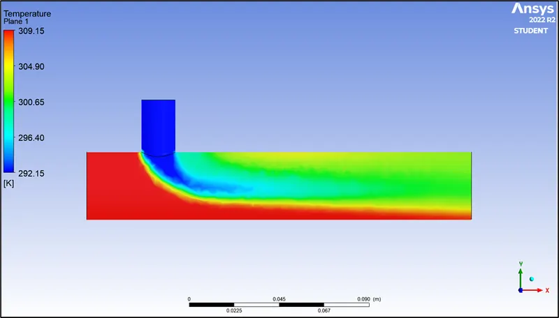
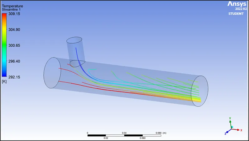
Temperature distribution across the plane:

Velocity distribution:

Velocity distribution across the plane:

Comparision:

	K-epsilon model	K-omega model
Area weighted average of temperature	30.28 (C)	30.34 [C]
Area weighted average of velocity	4.50(m/s)	4.50 (m/s)
Standard deviation of temperature	1.96(C)	2.20 (C)
Standard deviation of velocity	0.53(m/s)	0.59 (m/s)

Analytical Solution:

Mass of hot fluid (`m_h`) =`rho*a*v_h` = 1.225*0.0009*3= 0.0033075kg/s

Mass of cold fluid (`m_c`) =`rho*a*v_c`=1.225*0.0002*6= 0.00147kg/s

Temperature of mixture (`T_(mix)`)=`((m_h*T_h)+(m_c*T_c))/(m_c+m_h)` = 30.78 [C]

By comparing with Analytical solution k-epsilon model predicts the outlet temperature near to the analytical solution and effectiveness of mixing is 1.96 which is near to 1 and moreover K-epsilon model predicts well far from the boundaries and k-omega predicts well near the wall.Therfore k-epsilon model is majorily used for free flow away from the wall and as in this project their is no dealing with the wall of the mixing tee for change in temperature along the length,so k-epsilon model is choosen for further simulations.

CASE 1(B): SHORT MIXING TEE FOR M=4 (K-EPSILON MODEL):

we are using following inputs

Velocity of hot air at inlet=3 m/s

Temperature of hot air at inlet=36 (C)

Momentum ratio = 4

Momentum ratio= velocity of cold inlet/velocity of hot inlet

velocity of cold inlet = 12 m/s

Temperature of COLD air at inlet=19(C)

The procedure for this case also remains the same as explained earlier

OUTPUT:

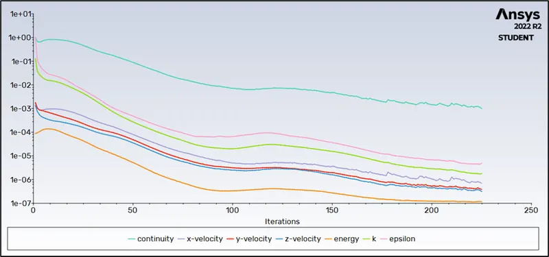
RESIDUAL PLOT:

CONVERGENCE PLOTS:

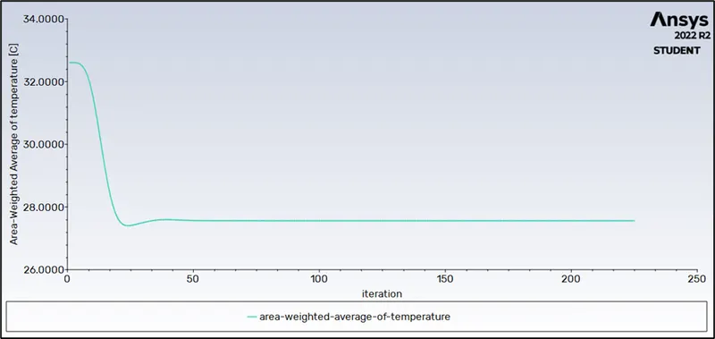
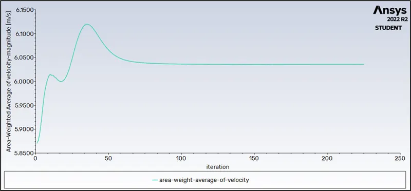
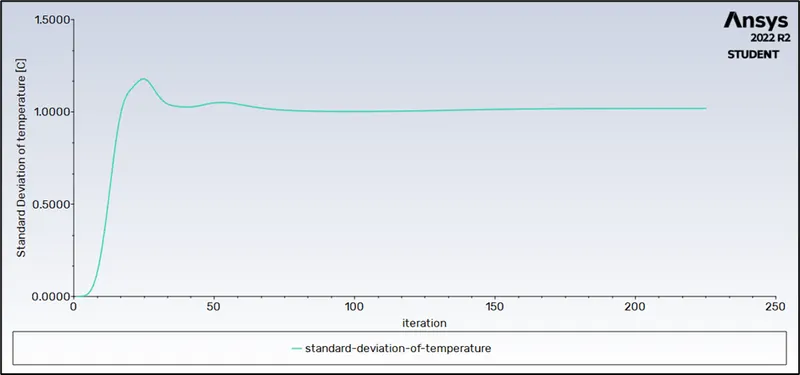
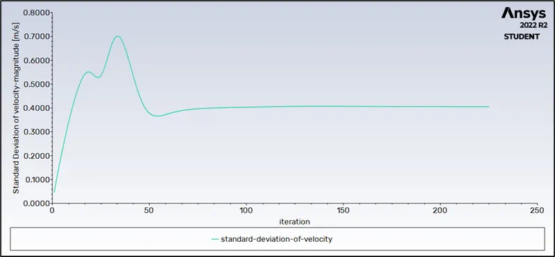
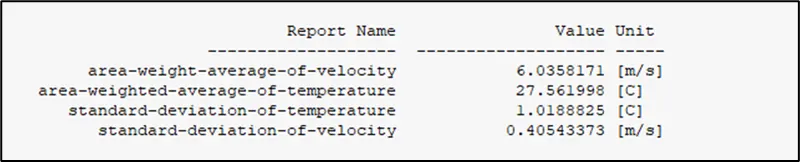
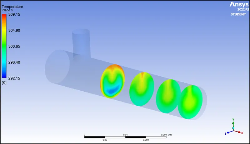
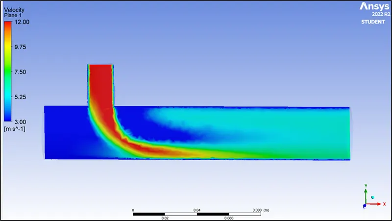
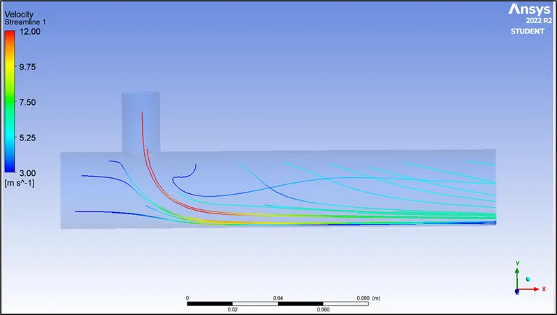
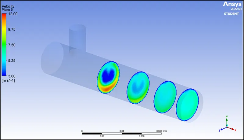
From above observation the average temperature and velocity at outlet is 27.56[C] Aand 6.03m/s respectively.

Temperature distribution:

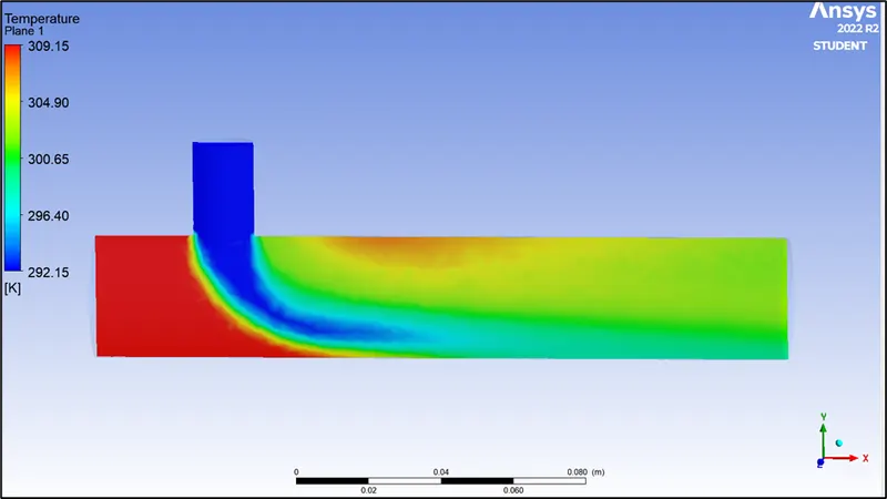
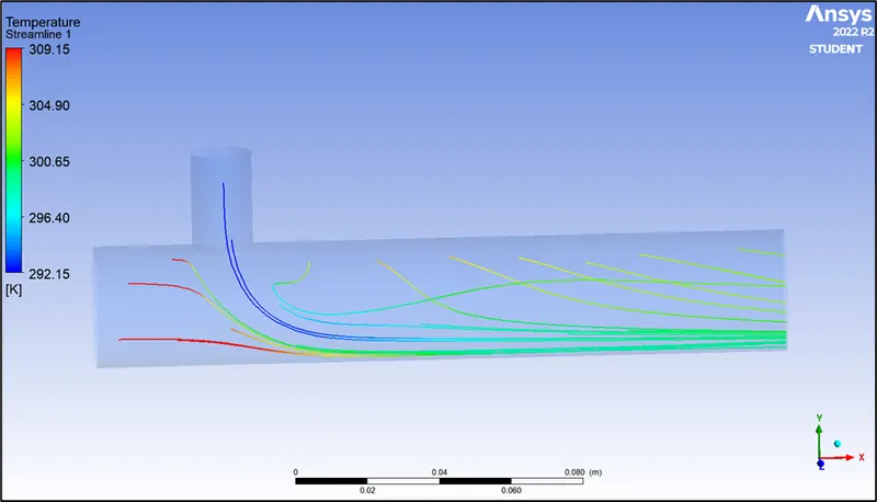
Velocity distribution:

Analytical Solution:

Mass of hot fluid (`m_h`) =`rho*a*v_h` = 1.225*0.0009*3= 0.0033075kg/s

Mass of cold fluid (`m_c`) =`rho*a*v_c`=1.225*0.0002*12= 0.00294kg/s

Temperature of mixture (`T_(mix)`)=`((m_h*T_h)+(m_c*T_c))/(m_c+m_h)` = 27.55 [C]

• Observation:

The Temperature at the outlet will be lesser than the one we got in the previous case. This is because the velocity of the cold air at the inlet is twice in this case when we compare it with the previous case. So, for the same length of the pipe, more amount of air is flowing through the inlet. The Mass flow rate has a formula of ρ⋅A⋅vwhere, v is the velocity of the fluid flowing. Since the velocity has increased, more mass will be flowing through the inlet therefore the temperature measured at the outlet will be even less.
This can be confirmed with our simulation results as well.

For M=4, the outlet temperature is approximately equal 27.56-degree celsius
For M=2, the outlet temperature is approximately equal to 30.34-degree celsius.

CASE 2(A): LONG MIXING TEE FOR M=2 (K-EPSILON MODEL):

we are using following inputs

Velocity of hot air at inlet=3 m/s

Temperature of hot air at inlet=36 (C)

Momentum ratio = 2

Momentum ratio= velocity of cold inlet/velocity of hot inlet

velocity of cold inlet = 6 m/s

Temperature of COLD air at inlet=19(C)

The procedure for this case also remains the same as explained earlier

OUTPUT:

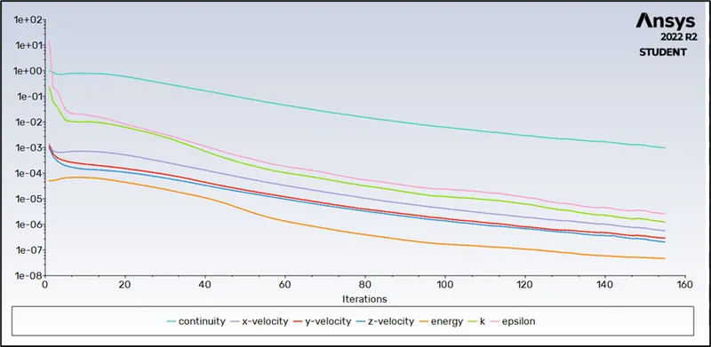
RESIDUAL PLOT:

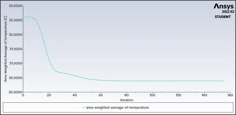
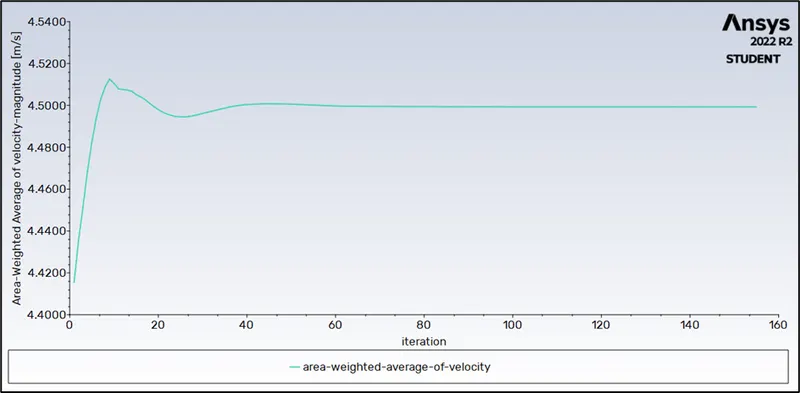
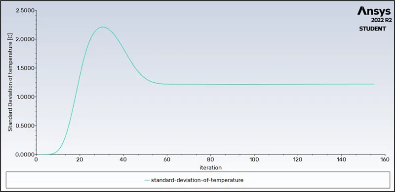
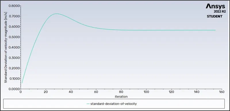
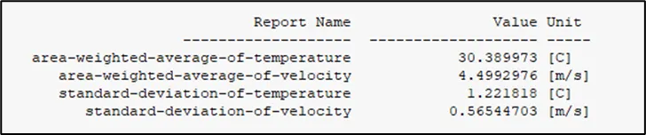
CONVERGENCE PLOTS:

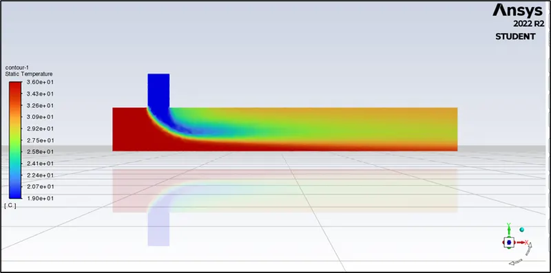
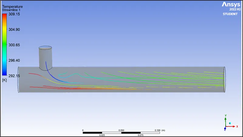
TEMPERATURE DISTRIBUTION:

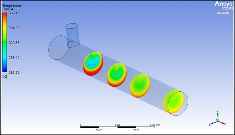
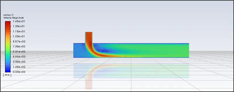
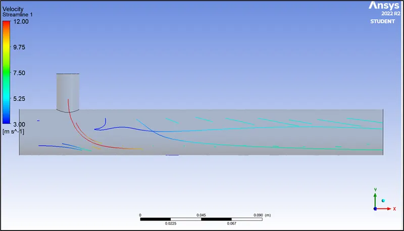
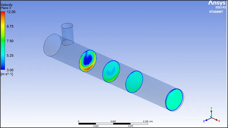
VELOCITY DISTRIBUTION:

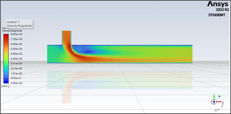
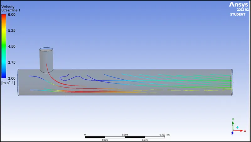
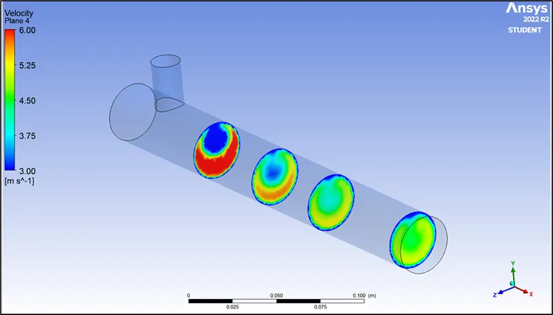
CASE 2(B): LONG MIXING TEE FOR M=4 (K-EPSILON MODEL):

we are using following inputs

Velocity of hot air at inlet=3 m/s

Temperature of hot air at inlet=36 (C)

Momentum ratio = 4

Momentum ratio= velocity of cold inlet/velocity of hot inlet

velocity of cold inlet = 12 m/s

Temperature of COLD air at inlet=19(C)

The procedure for this case also remains the same as explained earlier

OUTPUT:

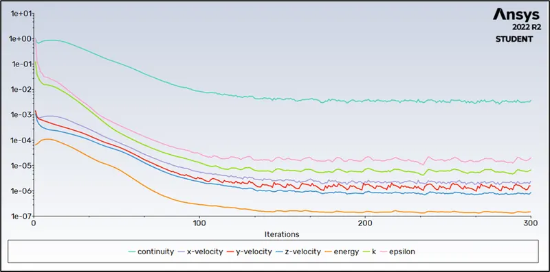
RESIDUAL PLOT:

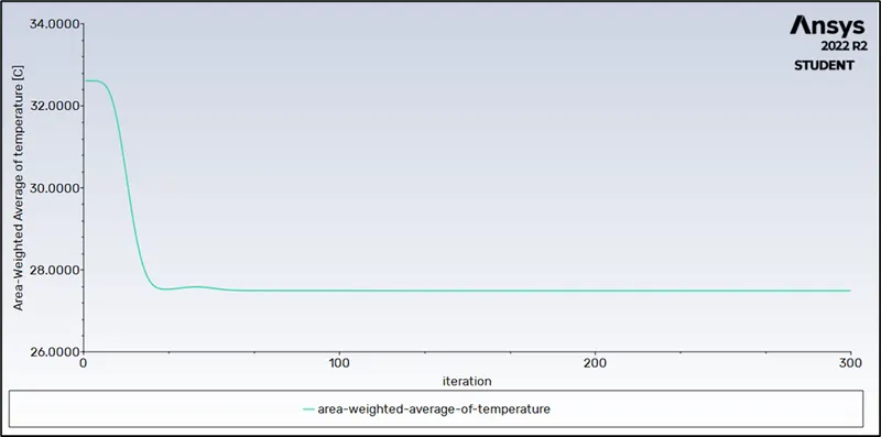
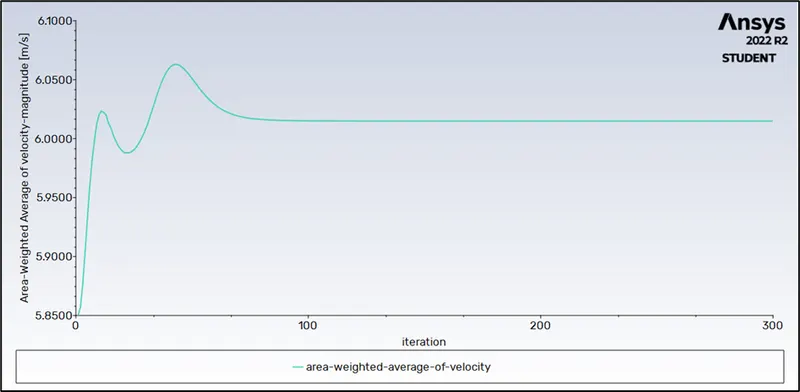
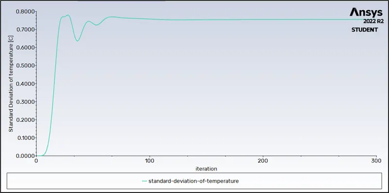
CONVERGENCE PLOTS:

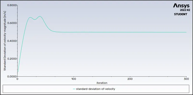
TEMPERATURE DISTRIBUTION:

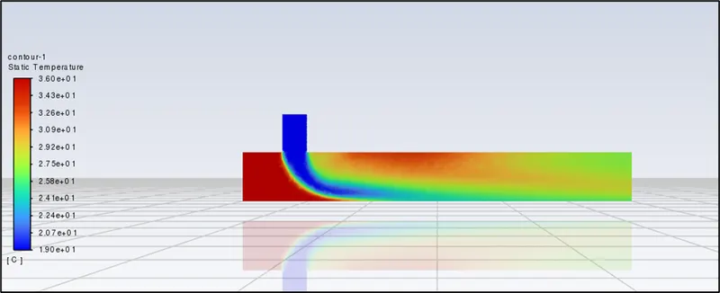
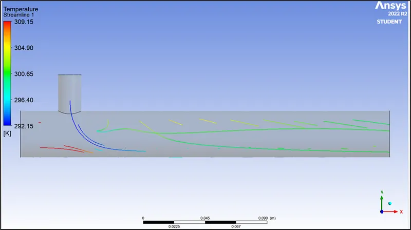
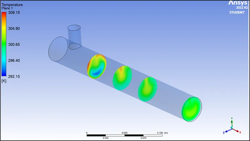
VELOCITY DISTRIBUTION:

• COMPARISION:

	MOMENTUM RATIO	AVERAGE OUTLET TEMPERATURE
MIXING TEE (SHORT)	M=2	30.34[C]
	M=4	27.56[C]
MIXING TEE (LONG)	M=2	30.38[C]
	M=4	27.48[C]

From the table, we can draw conclusions between the length of the Mixing pipe and the Momentum Ratio that we are using. We can see that for the same momentum ratio, there is no change in the output temperature with an increase in the length of the Mixing Tee.We can safely say that the length of the Mixing tee has no effect on the Output Temperature.
When we compare the Momentum Ratio is compared for the same length of the Mixing Tee, the increase in the momentum ratio results in a decrease in the Outlet Temperature because as the momentum ratio increases, the velocity of the Cold Air increases and due to this, the Mass flow rate increases thereby decreasing the Outlet Temperature of the air flowing out of the Mixing Tee. We can conclude that as the Momentum ratio increases, the Outlet velocity will increase.

• GRID INDEPENDENCE TEST:

The Grid Independence Test is done so as to check the dependency of the mesh on the Final Solution. The Accuracy will indeed change with the change of the mesh size, but the change in the accuracy should not be by a big margin.

We have taken three cases with a mesh size of 2mm,3mm & 4mm. The mixing Tee specifications are such that it is the Short Mixing Tee with a Momentum Ratio of 2 and have deployed the K-epsilon Turbulence Model for the simulation. We then compare the results that we get in these cases.

MIXING TEE (SHORT) ELEMENT SIZE	AVERAGE OUTLET TEMPERATURE
Element size = 2 mm	30.28[C]
Element size = 3 mm	30.25[C]
Element size = 4 mm	30.19[C]