Week 1- Mixing Tee

Aim:

To study T section which gives the desired outlet temperature, whether short or long. which Turbulence model captures the result efficiently for given momentum ratio.

Ansys Workbench:

• Geometry: The geometry of the project is loaded in here and control volume is extracted using space claim. It is used as a inbuilt clean up software.
• Mesh: The whole geometry is divided into no. of element to solve governing equation at every element.
• Setup: Here the input parameters for the boundaries, working fluid, report generation, solver selection, initialization and solution for the simulation is obtained.
• Solution: The entire solution for the the simulation is stored here.
• Result: This is used to post process the results of the entire simulation

Application of Mixing Tee:

• Water mixed with steam to preheat it before entering into boiler.
• Steam mixed with cold water to condense into liquid water.
• HVAC.

Baseline Simulation:

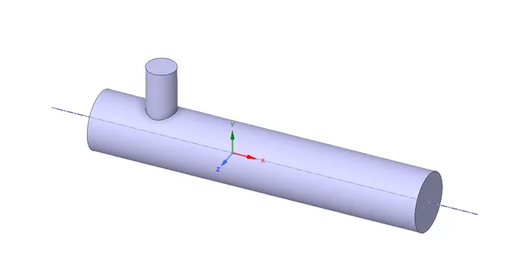
Geometry: using the Space claim the volume of fluid which is gonna be studied is extracted by selecting the edges of the model

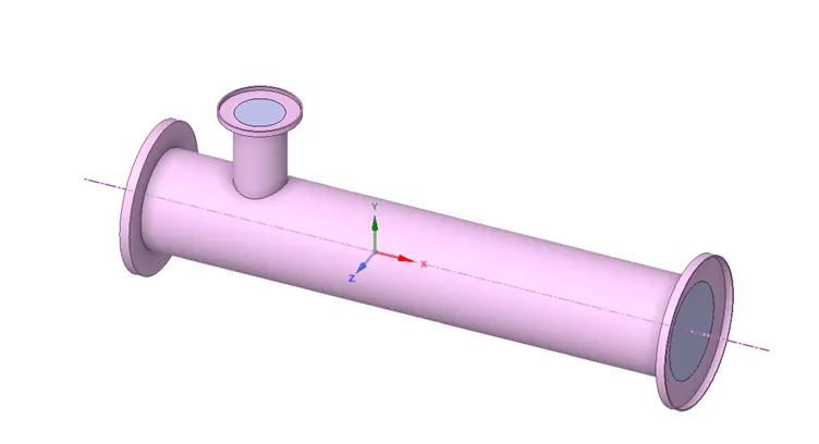
Extracted Volume:

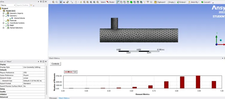
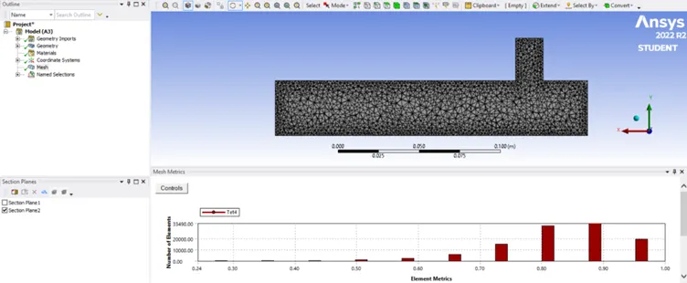
Mesh: Mesh generated over the entire geometry, then boundaries of the geometry is given names. The whole geometry is cut in half to seen the mesh within the geometry.

• Size:0.010219m
• Node: 2840
• Element: 12780

Named Selections:

• Inlet X: Inlet along the x direction.
• Inlet Y: Inlet along the Y direction.
• Outlet: Outlet along the x direction.
• Wall: The entire boundary of the extratced volume is selected

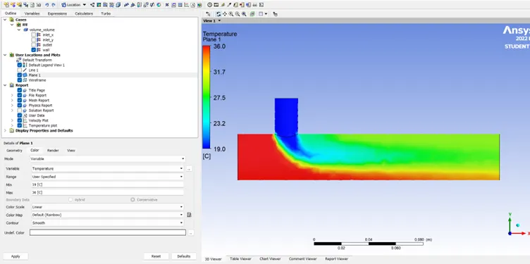
Contour:

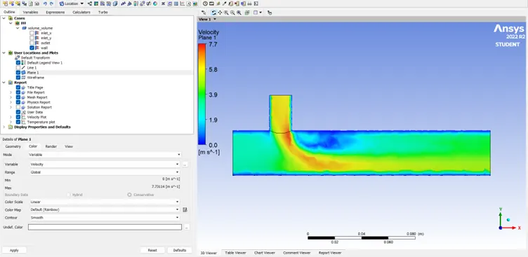
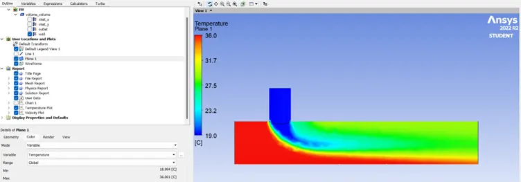
• This result is obtained in the post processing section, Within the Result post processing window select the Location toolbar plane give a name.
• From the left side thread line select the wall and double click, in the render option increase the transperancy.
• Select the plane and choose the Temperature option in the colour dialogbox, Similarly choose the velocity option to check the velocity distribution.

Tempertaure:

Velocity:

Plot:

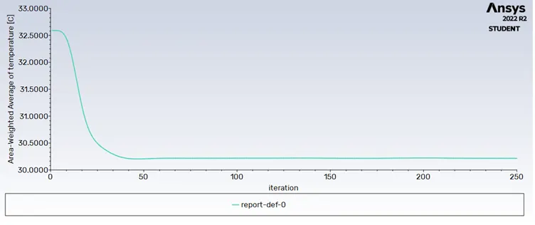
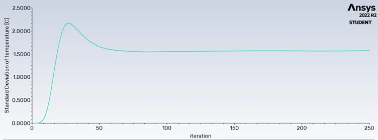
• This result is obtained from the report which is genertaed from the setup section.
• From the solution toolbar select the definition and click new, surface analysis then weighted average / std deviation.
• Select the boundary on which you need to calculate i.e. outlet.
• Then select both plot from bothom left corner, and click ok.

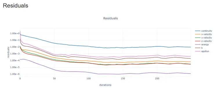
Residual:

Area Weighted Average at the Outlet: 30.2168*C

Standard Deviation: 1.572003*C

Temperature:

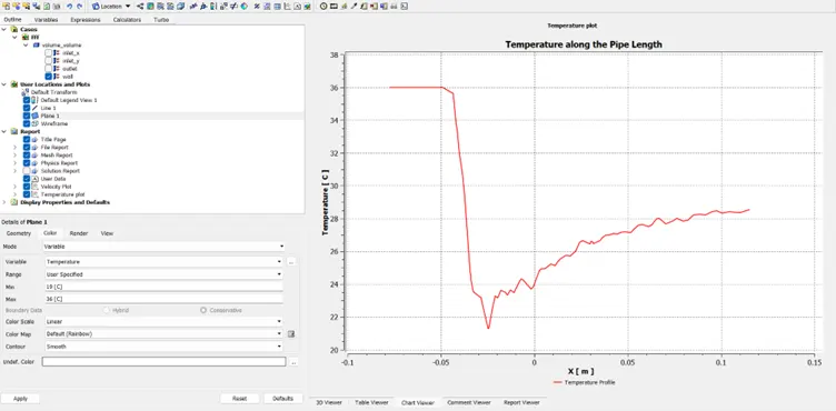
• This plot is obtained in the post processing Result section.
• Click on Location from the toolbar menu and select line, provide a name and select cut from the option.
• Select the graph symbol from the toolbar, provide name then from the dataseries select the line.
• Then from x axis select X from the option, from Y axis select the Temperature/Velocity and click apply to see the plot

Velocity:

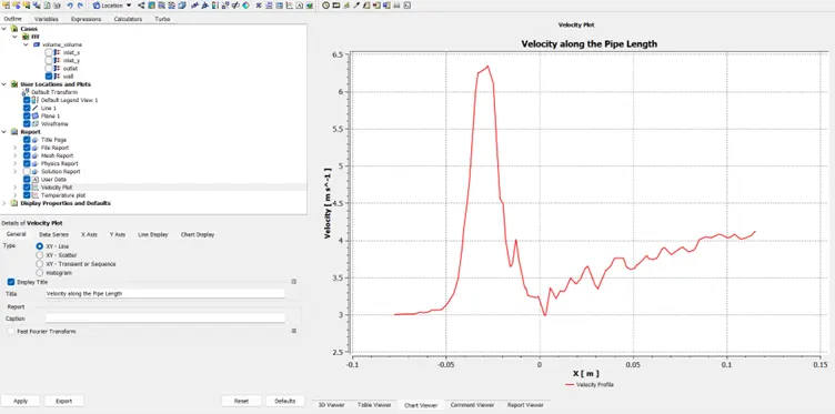
Conclusion: As the simulation have diffused result, this is due to the coarse mesh. Hence in actual simulation there is need for finer mesh.

Analytical Result:

`Tmix=((m(hot)*T(hot)) +(m(cold)*T(cold)))/(m(hot)+m(cold))`

• Tmix= mixing temperature of fluid,
• m(hot)= mass of hot fluid,
• m(cold)= mass of cold fluid,
• T(hot)= temperature of hot fluid,
• T(cold)= temperature of cold fluid.

mass of fluid(m)= `rho*A*V`

• rho= density of fluid.(for air = 1.225 Kg/m^3)
• A= area of geometry,
• V= velocity of fluid.

for, MR= 2

• A(hot)=901.3138mm^2, A(cold)=225.9823mm^2
• T(hot)=309.14*K, T(cold)=292.14*K
• V(hot)=3m/s, V(cold)=6m/s

`T(mix)=((1.225*901.3138*10^(-6)*3)*309.14+(1.225*225.9823*10^(-6)*6)*292.14)/((1.225*901.3138*10^(-6)*3)+(1.225*225.9823*10^(-6)*6))`

`T(mix)=303.462^circK=30.322 ^circC`

for, MR= 4

• A(hot)=901.3138mm^2, A(cold)=225.9823mm^2
• T(hot)=309.14*K, T(cold)=292.14*K
• V(hot)=3m/s, V(cold)=12m/s

`T(mix)=((1.225*901.3138*10^(-6)*3)*309.14+(1.225*225.9823*10^(-6)*12)*292.14)/((1.225*901.3138*10^(-6)*3)+(1.225*225.9823*10^(-6)*12))`

`T(mix)=300.6277^circK=27.4877^circC`

Case_1A_a: Short TEE

• Momentum Ratio = 2
• Inlet Temperature along the x axis = 36*C, flow velocity=3m/s
• Inlet Temperature along the x axis = 19*C, flow velocity=6m/s
• K – epsilon, realizable, wall standard function

Geometry: The geometry remains the same as that of the Baseline simulation.

Meshing:

• Size:.002m
• Node: 21457
• Element: 106587

Contour:

Temperature:

Velocity:

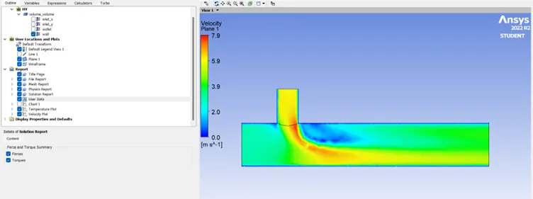
Plot:

Residual:

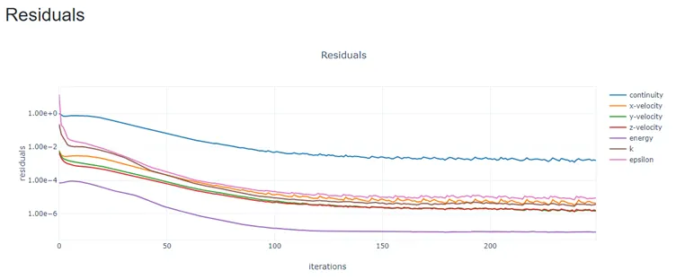
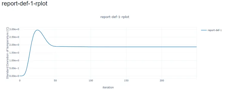
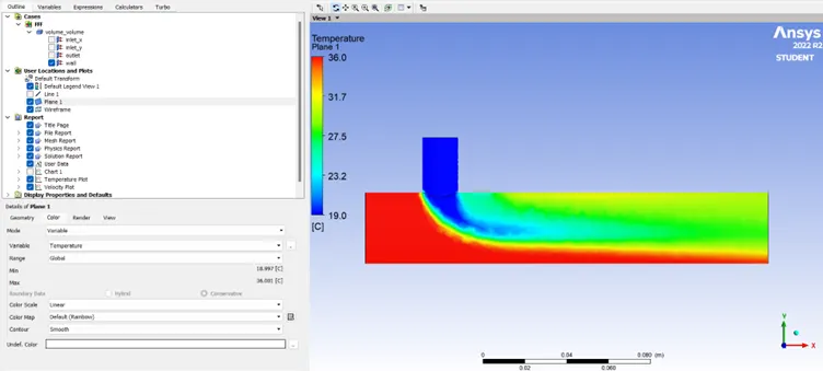
Standard Deviation of Outlet Temperature: 1.873044*C

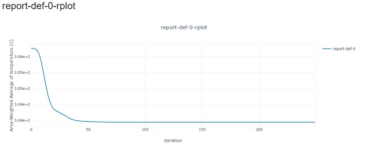
Area Weighted Average of Outlet Temperature: 30.29465*C

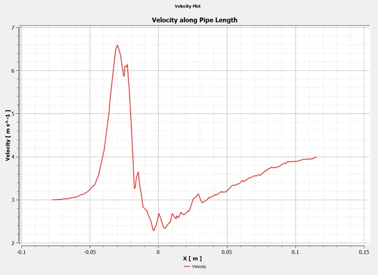
Velocity:

Temperature:

Case_1A_b:

• Momentum Ratio = 2
• Inlet Temperature along the x axis = 36*C, flow velocity=3m/s
• Inlet Temperature along the x axis = 19*C, flow velocity=6m/s
• K – omega, SST

Geometry: The geometry remains the same as that of the Baseline simulation.

Meshing:

• Size:.002m
• Node: 21457
• Element: 106587

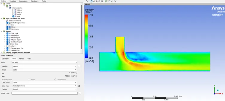
Contour:

Temperature:

Velocity:

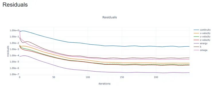
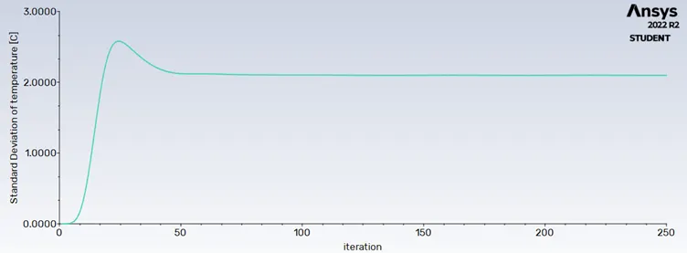
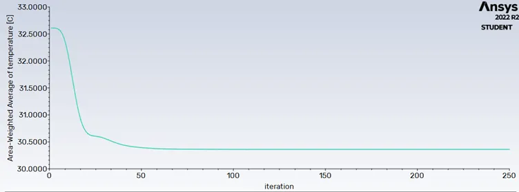
Plot: 250 iteration

Residual:

Standard Deviation of Outlet Temperature: 2.09756*C

Area Weighted Average of Outlet Temperature: 30.36042*C

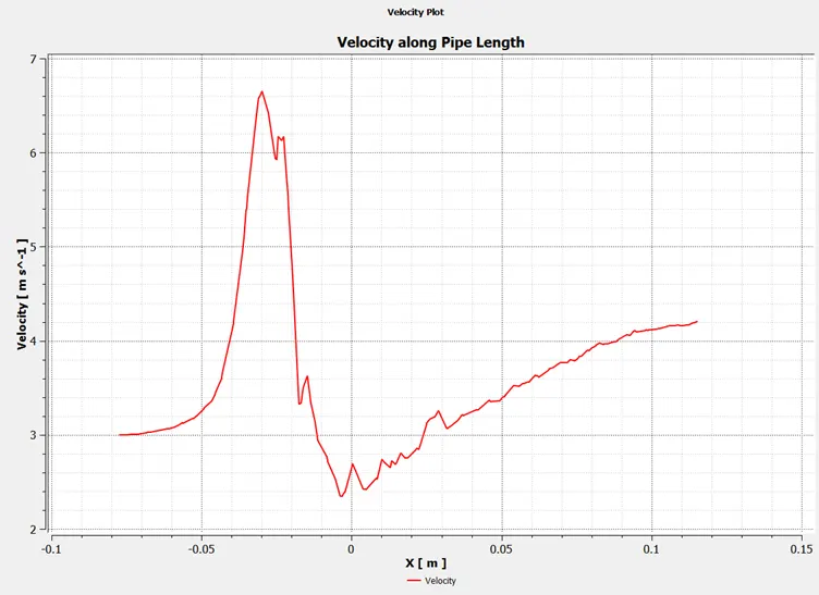
Velocity:

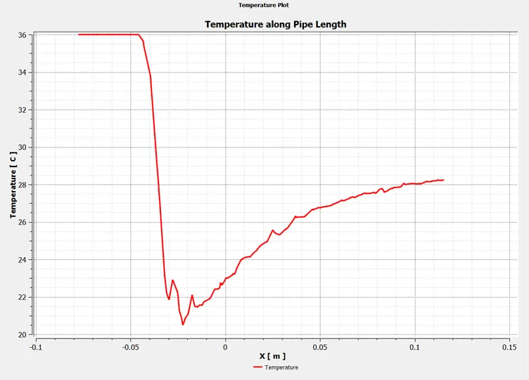
Temperature:

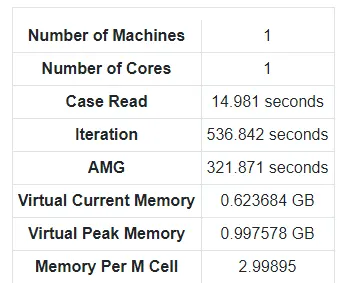
Conclusion :

1) K-Epsilon: 250+ iteration

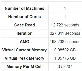
2) K-Omega : 250+ iteration

Case_1B_a:

• Momentum Ratio = 4
• Inlet Temperature along the x axis = 36*C, flow velocity=3m/s
• Inlet Temperature along the x axis = 19*C, flow velocity=12m/s
• K – epsilon, realisable, wall standard function

Geometry: The geometry remains the same as that of the Baseline simulation.

Meshing:

• Size:.002m
• Node: 21457
• Element: 106587

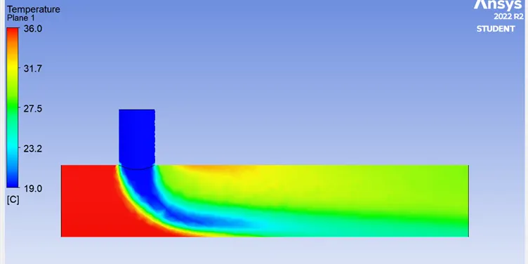
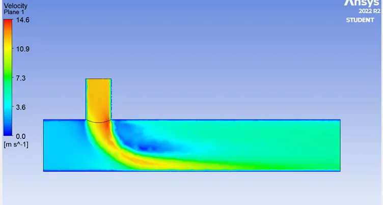
Contour:

Temperature:

Velocity:

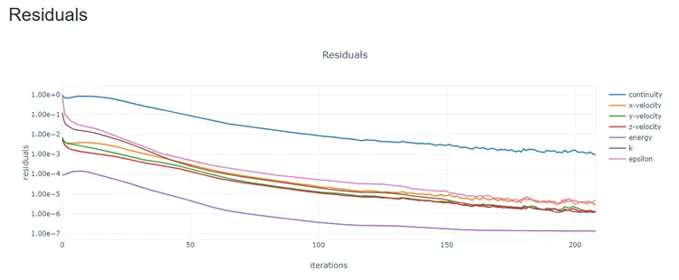
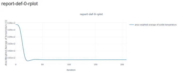
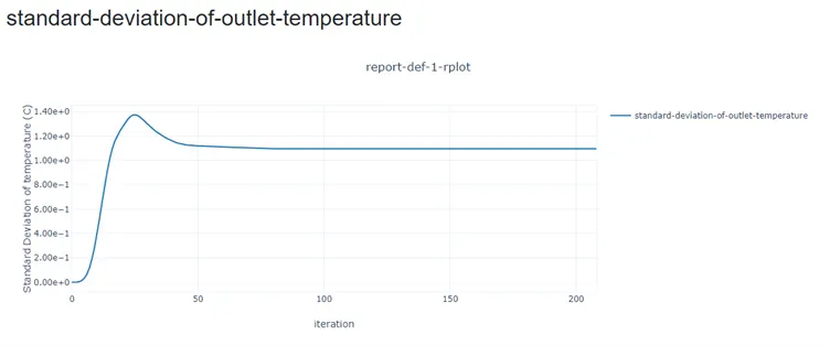
Plot: iteration 209

Residual:

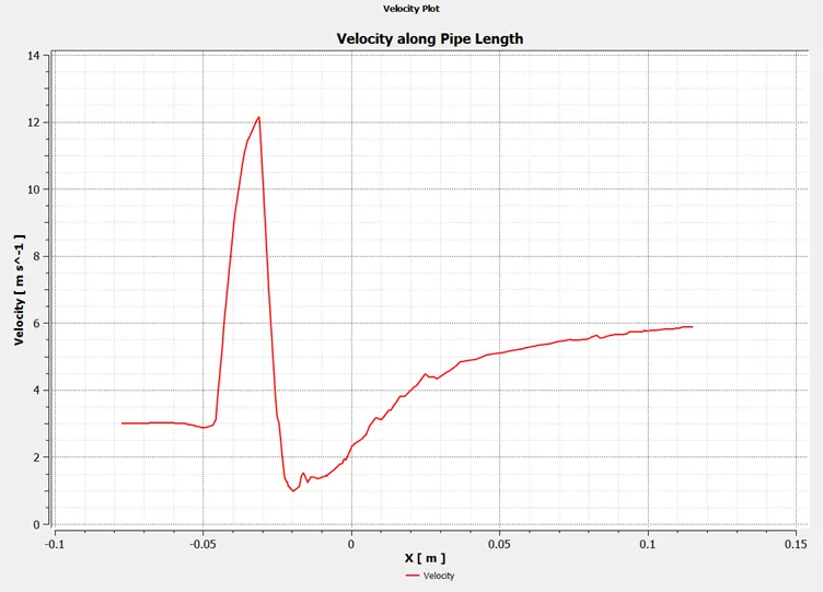
Area Weighted Average of Outlet Temperature: 27.57604*C

Standard Deviation of Outlet Temperature: 1.096733*C

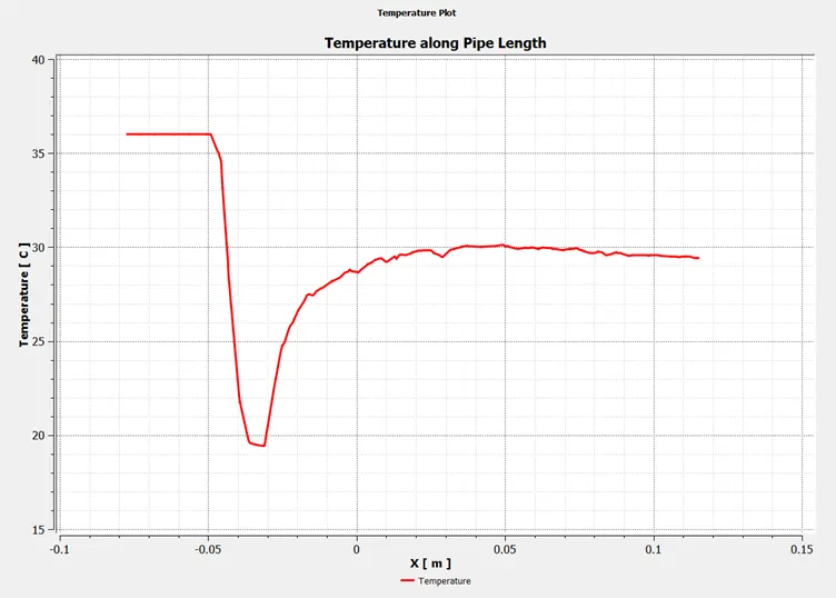
Temperature along the Pipe Length:

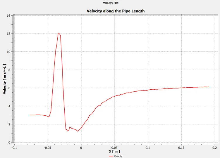
Velocity along the Pipe Length:

Case_1B_b:

• Momentum Ratio = 4
• Inlet Temperature along the x axis = 36*C, flow velocity=3m/s
• Inlet Temperature along the x axis = 19*C, flow velocity=12m/s
• K – omega, SST

Geometry: The geometry remains the same as that of the Baseline simulation.

Meshing:

• Size:.002m
• Node: 21457
• Element: 106587

Contour:

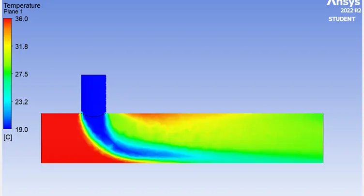
Temperature:

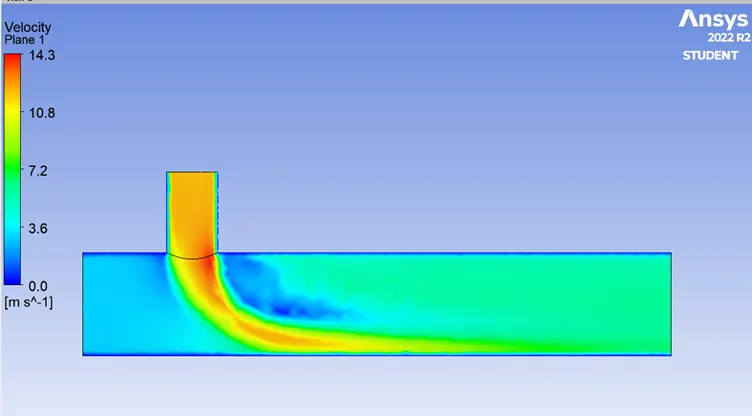
Velocity:

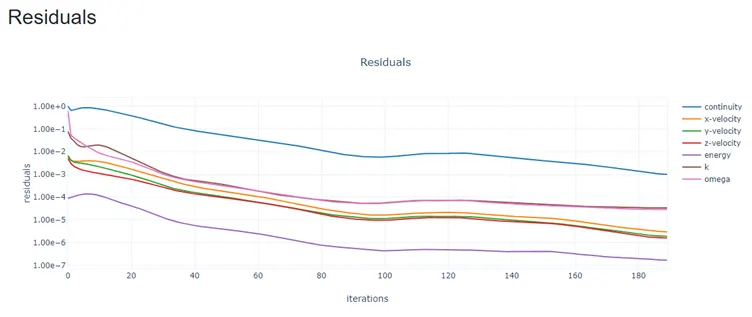
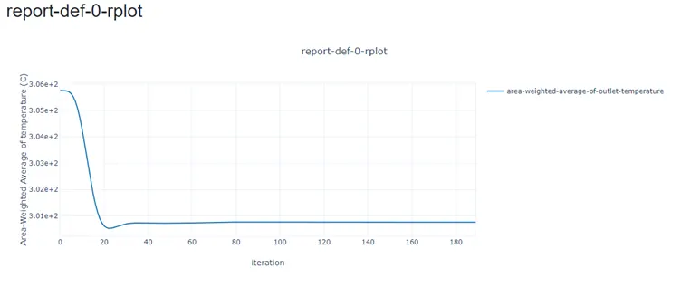
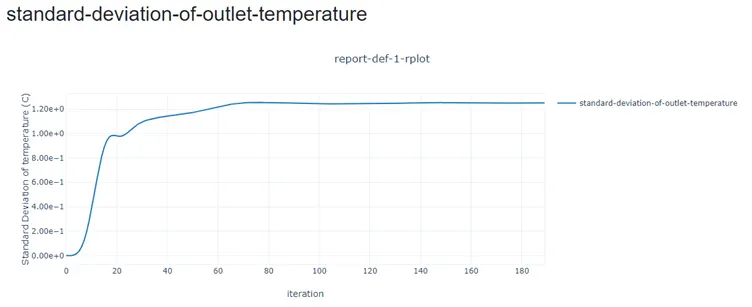
Plot: iteration 190

Residual:

Area Weighted Average of Outlet Temperature: 27.6068*C

Standard Deviation of Outlet Temperature: 1.25114*C

Temperature along the Pipe Length:

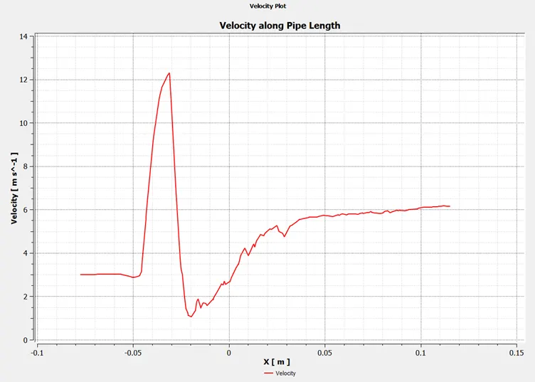
Velocity along the Pipe Length:

Conclusion :

1) K-epsilon : 209 iteration

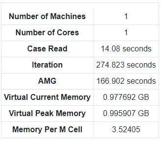
2) K-omega: 190 iteration

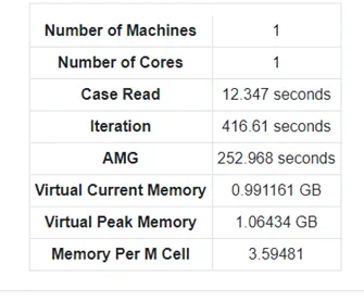
Even though the it took less iteration to solve using K-omega but the time taken by it to solve the solution is comparatively large.

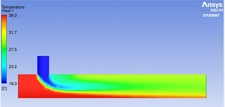
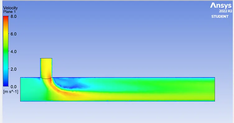
Case_2A: Long Tee

• Momentum Ratio = 2
• Inlet Temperature along the x axis = 36*C, flow velocity=3m/s
• Inlet Temperature along the x axis = 19*C, flow velocity=6m/s
• K – epsilon, realizable, wall standard function

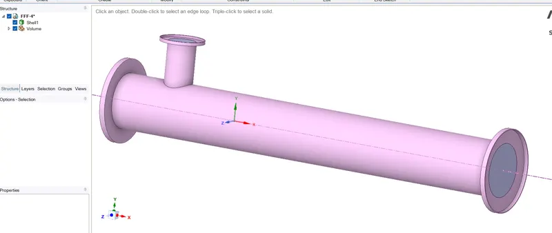
Geometry:

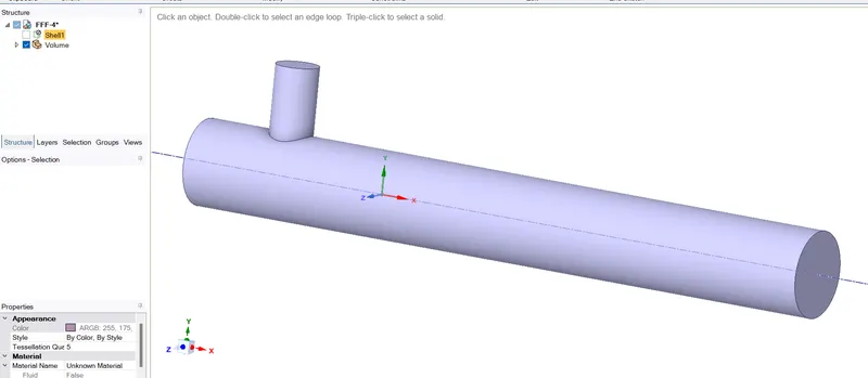
Volume Extracted:

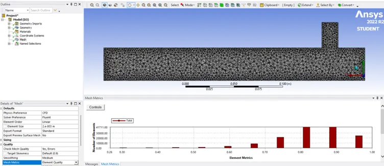
Meshing:

• Size:.002m
• Node: 28,450
• Element: 1,40,990

Contour:

Temperature:

Velocity:

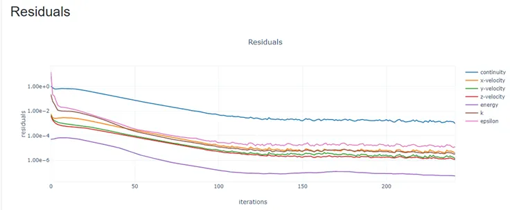
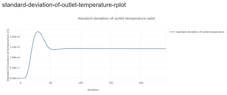
Plot: iteration 242

Residual:

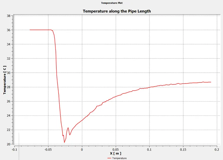
Area Weighted Average of Outlet Temperature: 30.37402*C

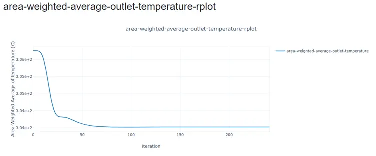
Standard Deviation of Outlet Temperature: 1.421174*C

Temperature along the Pipe Length:

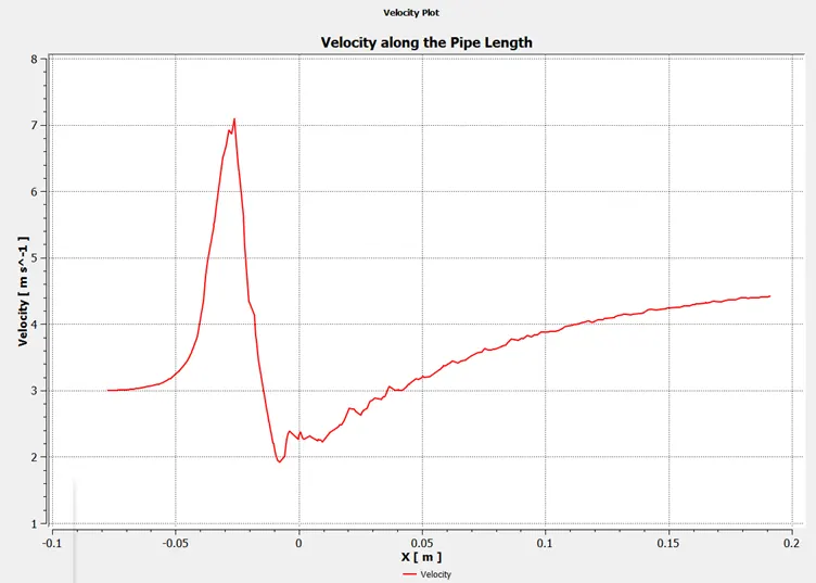
Velocity along the Pipe Length:

Case_2B: Long Tee

• Momentum Ratio = 4
• Inlet Temperature along the x axis = 36*C, flow velocity=3m/s
• Inlet Temperature along the x axis = 19*C, flow velocity=12m/s
• K – epsilon, realizable, wall standard function

Geometry: It is similar to Long tee with MR =2

Meshing:

• Size:.002m
• Node: 28,450
• Element: 1,40,990

Contour:

Temperature:

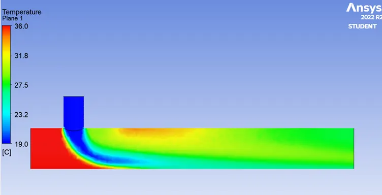
Velocity:

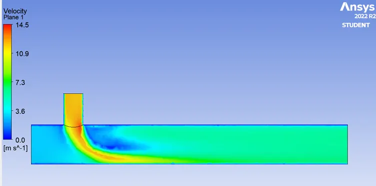
Plot: iteration 219

Residual:

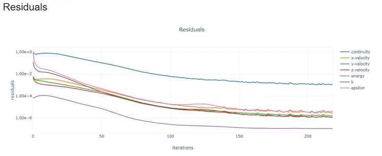
Area Weighted Average of Outlet Temperature: 27.49174*C

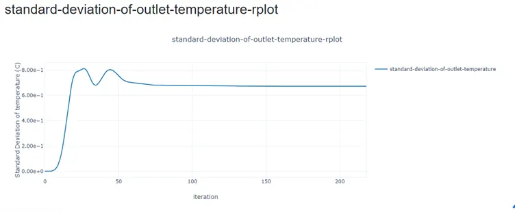
Standard Deviation of Outlet Temperature: 0.6723908*C

Temperature along the Pipe Length:

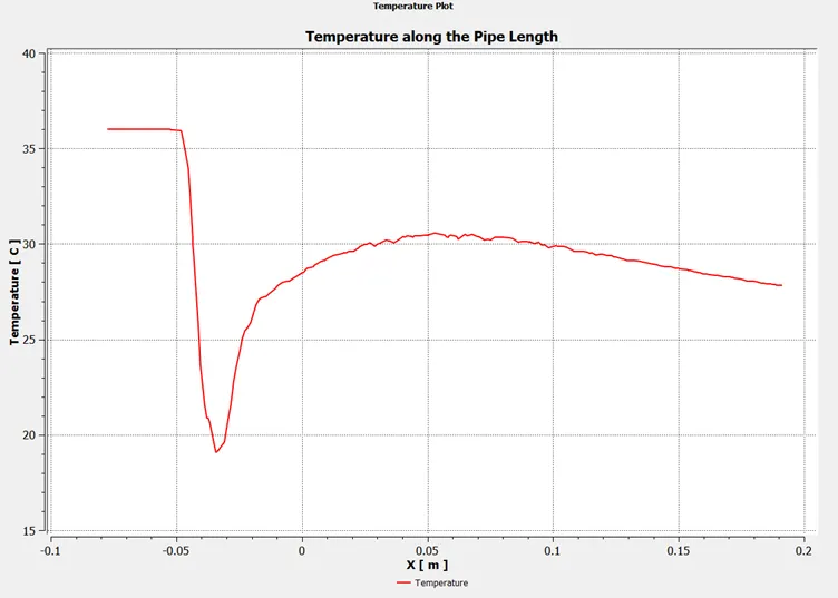
Velocity along the Pipe Length:

Conclusion:

1) K-epsilon : 242 iteration

2) K-epsilon: 219 iteration

• Time taken to solve the Long Tee with small MR takes more time and iteration to solve than with higher MR.

Mesh Independence test:

Sr. No.	Element Size	Temperature	Standard Deviation
	0.0015	30.33698*C	2.130153*C
1	0.0025m	30.2935*C	1.706762*C
3	0.0035m	30.2724*C	1.526191*C
2	0.005m	30.26245*C	1.342026*C

From the above data it is clear that the temperature for all the element size is similar with less deviation. Hence it is clear that the solution for the problem does not depend on the mesh size.

Final Result: In order to compare the results of all the method in one go, one must select Result table from component system and drag adrop at desrired location. then select the solutions of the desired simulation and drop it into the result table, Like wise do the same for the simulation which you need to compare the results.

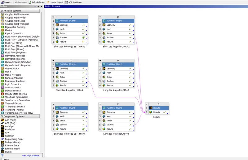
1) Comparing Temperature, the long Tee for MR= 2,4:

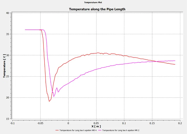
• Comparing the temperature, we see that the as the MR is increased Fluid mixing takes place very efficiently within shorter length.
• Inorder to increase the effectiveness of fluid mixing, higher MR is preferred.

2) Comparing the velocity of Long Tee:

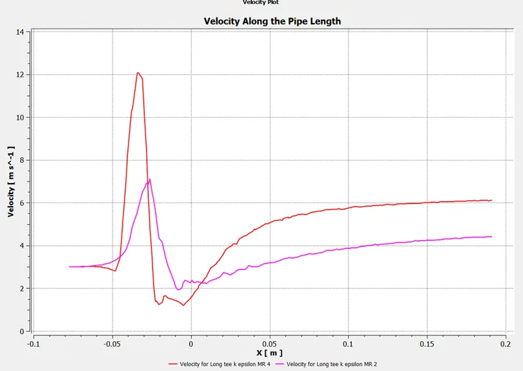
• With the increased MR the overall outlet velocity of fluid is also increased.

3) Comparing Short & Long Tee temperature along the pipe length:

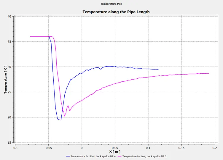
• As we increase the MR, length of the mixing pipe could be reduced.

Cumulative Result:

Parameter	Solver	MR	Analytical Temperature	Numerical Temperature	% Error	Numerical STD Deviation	No. of Iteration	Time to Solve Iteration	No. of Element
Short Tee	K-Epsilon	2	30.322*C	30.29465*C	0.0902	1.873044*C	250+	327.31sec	106587
	K-Omega	2		30.36042*C	0.1267	2.09756*C	250+	536.842sec
	K-Epsilon	4	27.4877*C	27.57604*C	0.3214	1.096733*C	209	274.823sec
	K-omega	4		27.6068*C	0.4332	1.25114*C	190	416.61sec
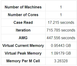
Long Tee	K-Epsilon	2	30.322*C	30.37402*C	0.1715	1.421174*C	242	715.785sec	140990
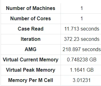
	K-Epsilon	4	27.4877*C	27.49174*C	0.01469	0.6723908*C	219	372.23sec

• From the above table it is clear that from both K-Epsilon & K-omega Error obtained is similar, further the computational time taken for the K-Omega method is longer than K-Epsilon method. Hence for this simulation we choose to use k-Epsilon Realisable, standard wall function method.
• Now, comparing between MR 2 & 4, for both long and short TEE the computational time taken for MR 2 is large eventhough no. of element being same. If selection need to be made between MR=2 & 4, then 4 would be correct choice as the STD deviation value is smaller for MR=4, which means the air is mixed efficiently.
• Comparing between Long & Short TEE for same MR, with longer TEE mixing of air takes more efficiently while the computational time is large as the no. of element being large. So, for same MR Long TEE would be the best choice.
• Comparing between Long TEE MR=2 & Short TEE MR=4, eventhough the % error is large for short TEE but the air is mixed efficiently with less computational time. Hence Short TEE with high MR value being the best choice, as this helps to make compact and economical design.
• Comparing between Long TEE MR=4 & Short TEE MR=2, for this longer tee would be the best choice as the computation time being similar, % error being low, and STD. deviation being low. Longer tee with high MR is best choice when mixing is more importatnt then compactness or economical.