Week 1- Mixing Tee

MIXING TEE-

AIM- To perform a steady state simulation in order to observe mixing of fluids in Tee joints by varfying length of joint as well as by varying inlet velocity at hot and cold inlets.

1. Case 1
   • Short mixing tee with a hot inlet velocity of 3m/s.
   • Momentum ratio of 2, 4.
2. Case 2
   • Long mixing tee with a hot inlet velocity of 3m/s.
   • Momentum ratio of 2, 4.

Momentum ratio = velocity at cold inlet / velocity at hot inlet

Procedure-

Setting up geometry and Mesh-

Start with setting up geometry in ansys fluent. Upload geometry in Ansys fluent.

2. Remove thickness from geometry as we need only volume where fluid flows.

3. Surpress extra volume so that no equations are solved in those areas.

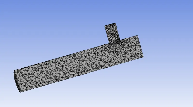
4. Create mesh after creating volume and create a cut plane too see full view of mesh.

5. After that comes setting up boundary conditions and simulation parameters like turbulence models, steady state simulations, energy equations etc.

6. run simulation and check post process results.

Geometry-

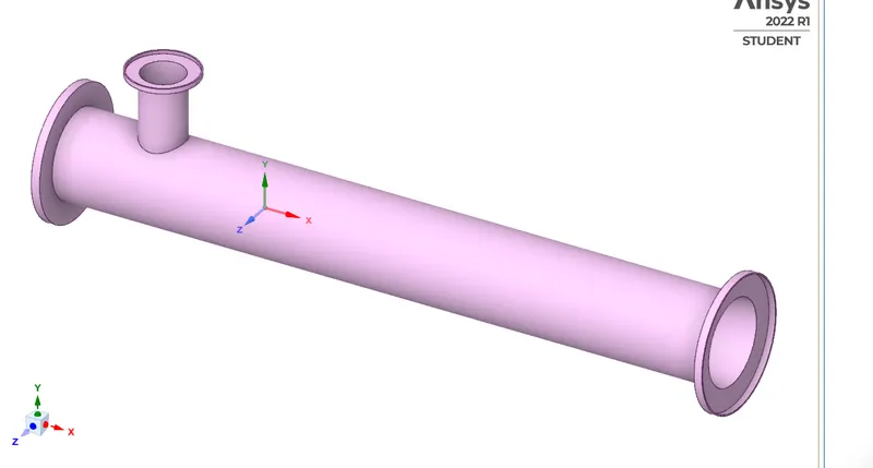
Two type of geometry is used in this simulation

-Mixing tee short length

-Mixing tee long length

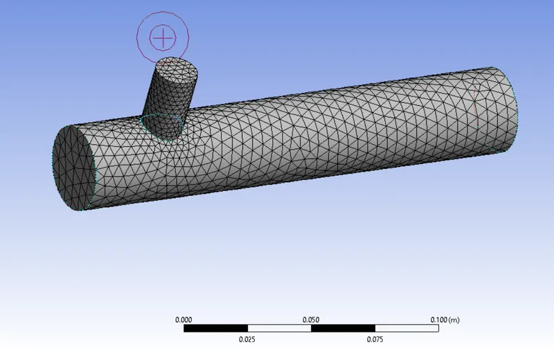
Mesh generated

Start with default value for mesh element size.

Creating cut plane

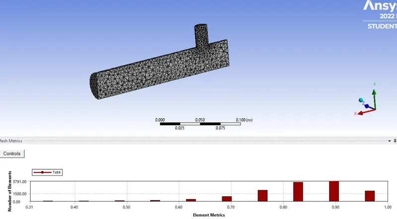
Checking Mesh quality-

After creating mesh it is required to check mesh quality and no mesh elemnt goes below desired value. Minimum mesh quality is above 30 percent so we are good to go.

Setting up Simulation-

1. Setting up simulation includes identifying boundaries and defining boundary conditions.

2. Simulation is steady-state. Two turbulence models K-epsilon and K-omega are used in simulation for two different cases.

3. Boundary conditions-

Case 1. for both short Tee and long Tee

Turbulence model- K-epsilon

Inlet X- Velocity inlet - 3m/s

Inlet Y- 6m/s

Outlet- Pressure-velocity

Body- Wall boundary condition

Case 2. for both short and long Tee

Inlet X- velocity inlet- 3m/s (hot )

Inlet Y- Velocity inlet- 12m/s

Walls- boundary type wall

Mixing-Tee short

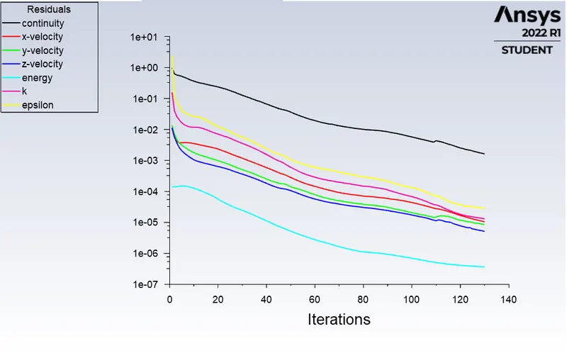
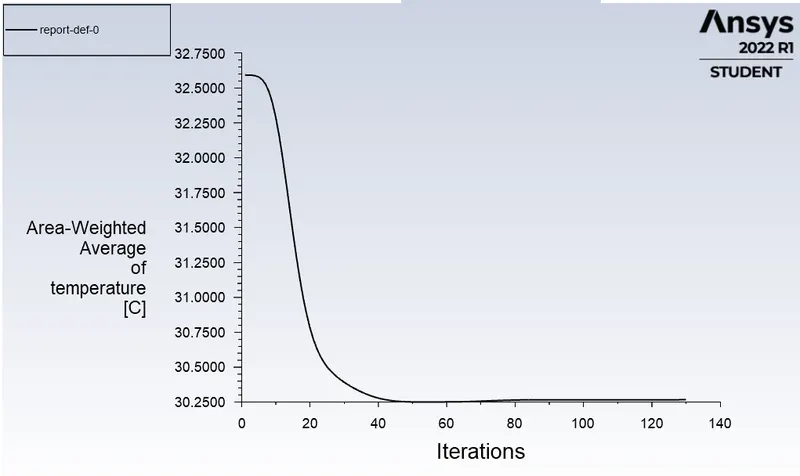
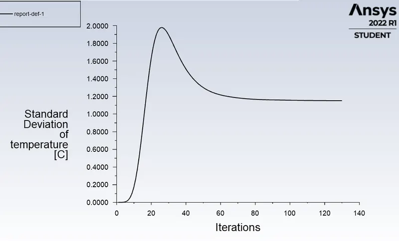
Case 1-

Case-2

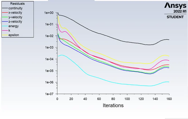
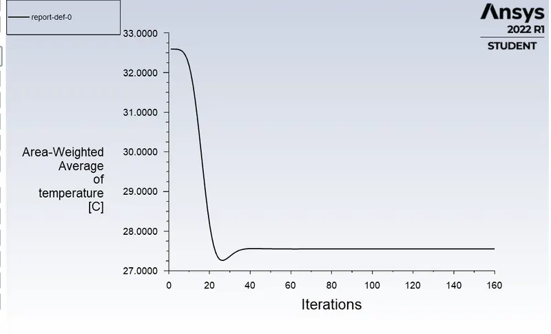
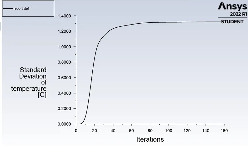
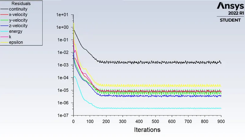
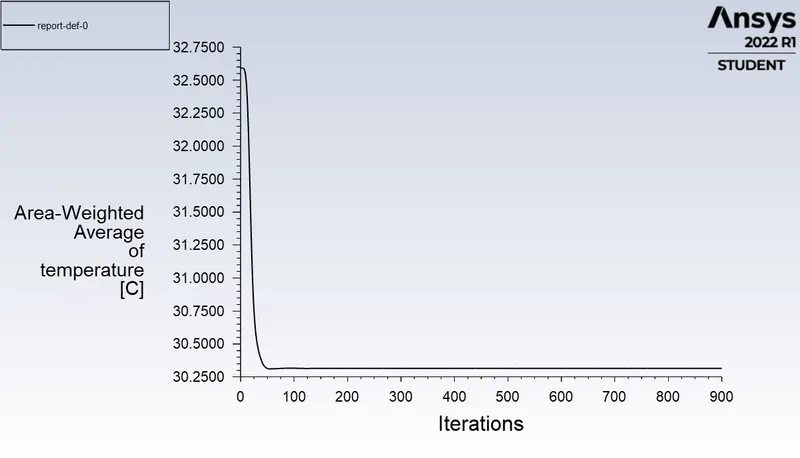
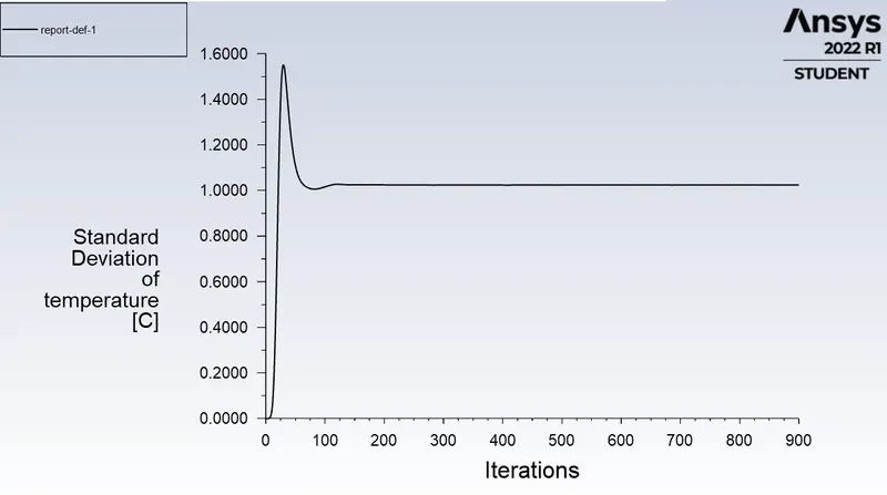
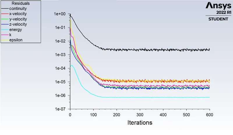
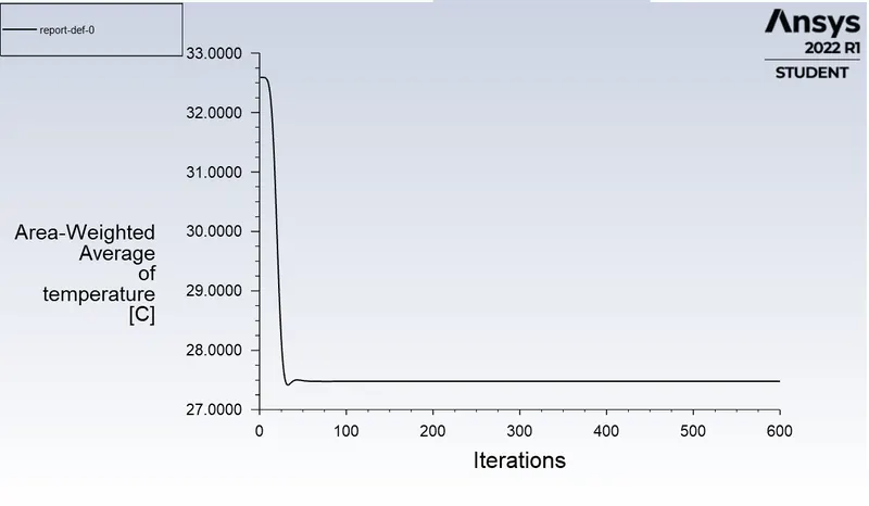
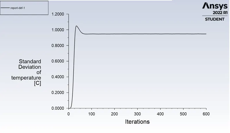
• Value for above posted results are not converged as number of iterations used is low so atleast keep iteration number upto 1000 so that solver gets enought time to give converged results.
• Above given plots are for K-epsilon Turbulence model

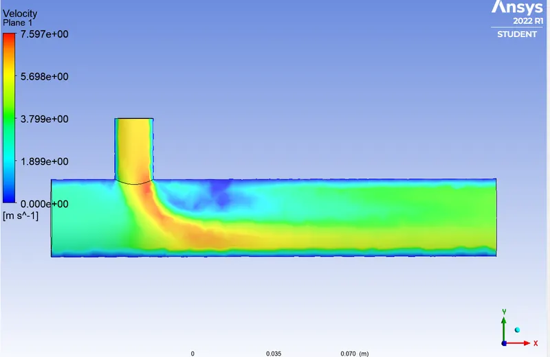
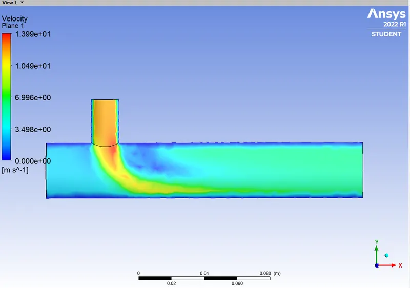
Velocity Contour Short-tee

Case 1- Momentum2

Case2- Momentum 4

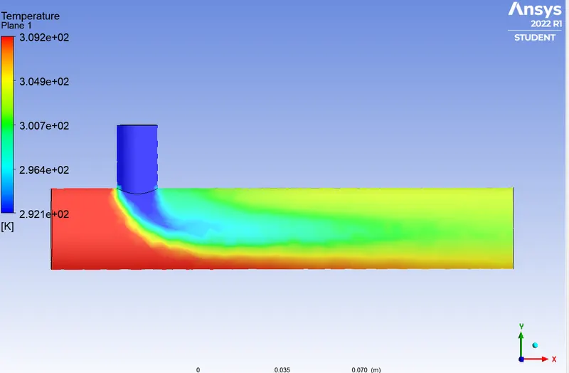
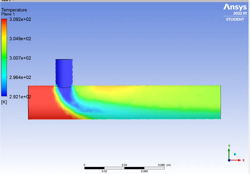
Temprature Contour short-tee

Case-1 Momentum 2

Case-2 Momentum 4

Mixing-Tee long

Case 1 momentum 2

Case 2 momentum 4

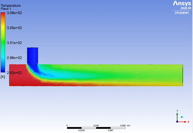
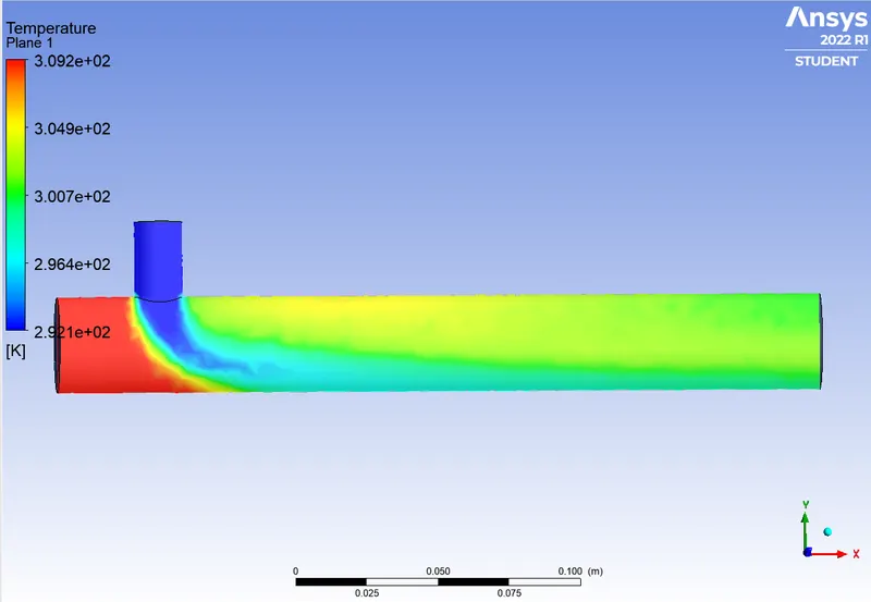
Temprature contour

Case 1 Momentum 2

Case-2 Momentum 4

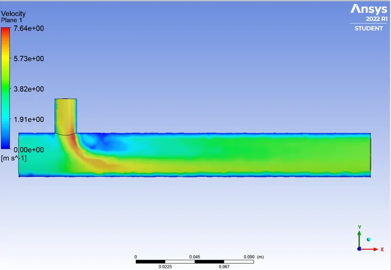
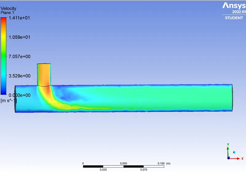
Velocity contour

Case 1 Momentum 2

Case 2 Momentum 4

Comparing following three parameters in a table-

1. Cell count
2. Average outlet temperature
3. Number of iterations for convergence

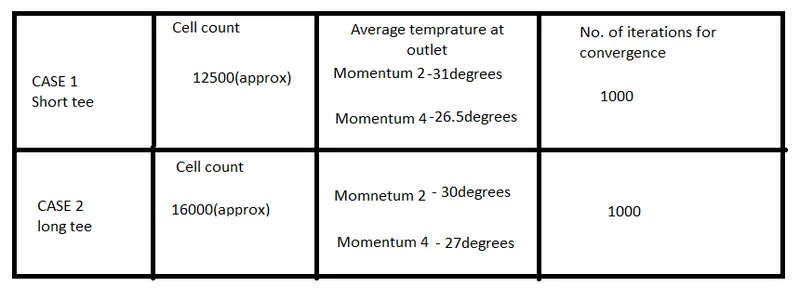
Conclusion-

Velocity contour of short tee for case 1 & 2

• Formation of zero velocity region is more for case 1 as compared to case 2.
• Mass flow rate for cold air increases for case 2 which fills teee with more cool air at higher velocity which resulted in decrease of velocity at oulet in case 2 as compared to case 1.

Velocity contour of Long tee for case 1 & 2

• Velocity inside tee for case 2 is lower as compared to case 1 because of increase in velocity from Inlet-Y, flow rate for cold air is more than that of hot air. At oulet temprature is lower than outlet.

Temprature contour of short tee for case 1 & 2

• Temprature at outlet decrease but mixing of cold and hot air is not proper because of short length of tee.

Temprature contour of long tee for case 1 & 2

• Cold and hot air properly mixed as sufficient length is provided for both to get mixed.
• Area of hot air is decreased with increase in velocity incoming cold air.