Week 1- Mixing Tee

OBJECTIVE:- Our objective is to set up steady-state simulations of a T-Joint mixing to compare the mixing effectiveness when hot inlet temperature is 36⁰C and Cold inlet is at 19⁰C. We use the k-epsilon and k-omega SST model for our first case and based on this observation, we use the more suitable model for further cases.

Case 1

• Short mixing tee with a hot inlet velocity of 3m/s.
• Momentum ratio of 2, 4.

Case 2

• Long mixing tee with a hot inlet velocity of 3m/s.
• Momentum ratio of 2, 4.

Where Momentum ratio = (velocity at the cold inlet)/(velocity at the hot inlet)

DESCRIPTION OF THE PROJECT:- Mixing tees—in which two fluid streams with different physical or chemical properties mix—are widely used in the industry and mainly the petrochemical industry. When there is a large temperature difference between two streams, large metal temperature fluctuations can occur in the region where the two streams meet if proper design steps are not taken. Here we mixed up two fluids which are in different temperatures. One fluid is 36C, another is at 19C and we see the temperature at the outlet. And we also visualize how the temperature fluctuates from the mixing point to the outlet of the pipe.

In the first case, to simulate the mixing tees flow we will take two models to examine which one is better performing, and based on those results we will further proceed, the two models are-

1. K-omega model:- The k-omega (k−ω) turbulence model is one of the most commonly used models to capture the effect of turbulent flow conditions. It belongs to the Reynolds-averaged Navier-Stokes (RANS) family of turbulence models. It is a two-equation model. That means in addition to the conservation equations, it solves two transport equations (PDEs), which account for the historical effects like convection and diffusion of turbulent energy. The standard k−ωmodel is a low Remodel, i.e., it can be used for flows with low Reynolds number where the boundary layer is relatively thick and the viscous sublayer can be resolved. Thus, the standard k−ω model is best used for near-wall treatment.
2. K-epsilon model:- K-epsilon (k-ε) turbulence model is the most common model used in Computational Fluid Dynamics(CFD) to simulate mean flow characteristics for turbulent flow conditions. It is a two-equation model that gives a general description of turbulence using two transport equations (Partial Differential Equation, PDEs). The original impetus for the K-epsilon model was to improve the mixing length model, as well as to find an alternative to algebraically prescribing turbulent length scales in moderate to high complexity flows. k- epsilon model predicts well far from the boundaries (wall).

Again the selection of the model depends on the specific problem, no turbulence model is suited for every case. Fine-tuning is required.

For simulation, we have to go through some steps –

1. First, we import or create our geometry in the Ansys Fluent
2. Then, we prepare our geometry
3. Then we go for meshing. After doing the meshing, we give the name of every portion like inlet, outlet, and wall.
4. Next, we go for results. We give the initial and boundary condition. We also give the iteration number and then, we run the calculation.
5. The last step is post-processing.

In this simulation, in the case of results, we see the residuals plot, Area-Weighted Average of the temperature plot for the outlet face, and Standard Deviation of the temperature plot of the outlet face.

CASE-1:- Here we use short mixing tee for our simulation

1. A) In this case, the momentum ratio is 2, which means hot inlet velocity is 3m/s and cold inlet velocity is 6m/s. And the hot inlet temperature is 36`℃` and the cold inlet is 19`℃`. Here, we use K - Epsilon model for simulation:-

GEOMETRY:-

This is the geometry we have -

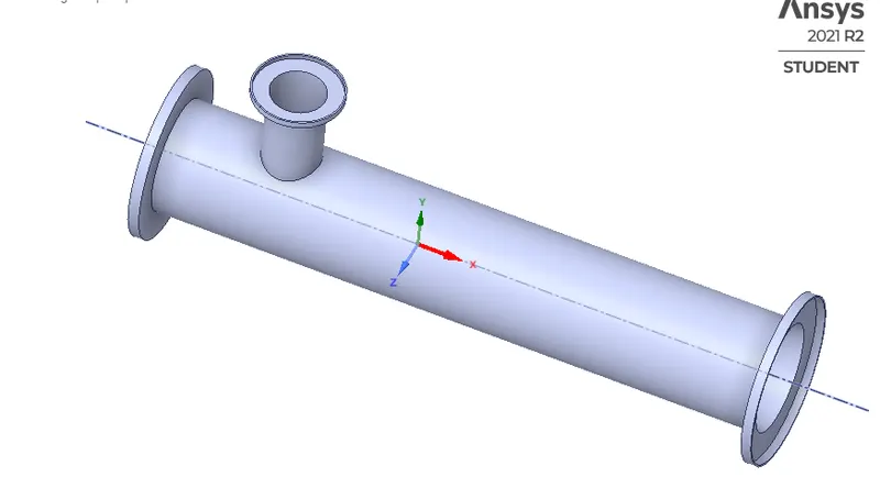
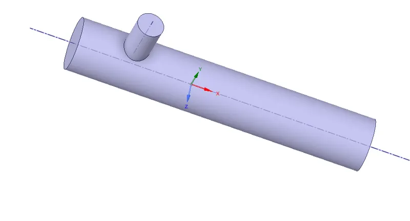
Here we only required the extracted volume of this geometry. So, we extracted it's volume by using Spaceclaim's one of the best features volume extracted by selecting edge's of the geometry.

MESH:- Meshing is a very important part of any simulation. With the increasing of meshing elements, the accuracy of the solution is increasing. We created our mesh and here we use the tetrahedrons method to generate the mesh.

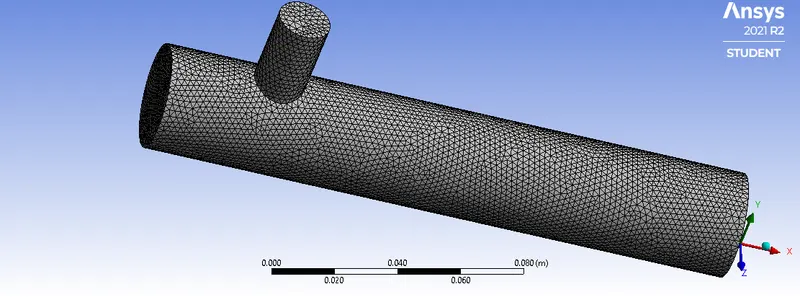
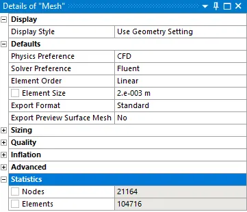
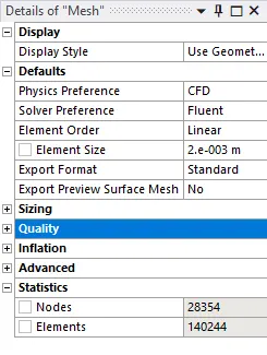
The element size of the mesh is 0.002. Here is the all details of the mesh -

Quality check of our mesh - Ansys has a inbuilt mesh quality checking function.

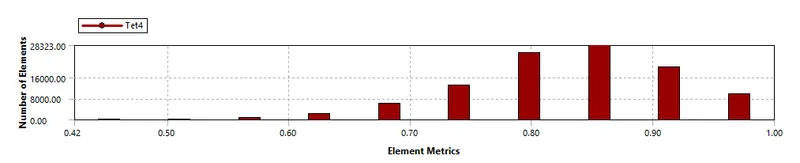
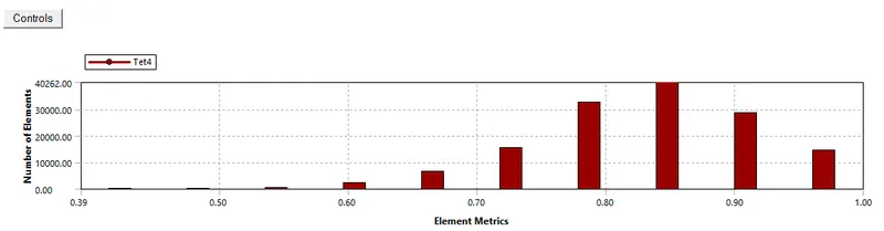
After, seeeing this graph we can say that our mesh is quite good for simulation.

Now we go for the simulation part. After settting up all the physics, initial condition and boundary condition we are going for results.

But before we start our calculation or patch initial values for selected variables in selected cells we must initialize the flow field in the entire domain. The solution initialization task page allows us to set initial values for the flow variables and initialize the solution using these values. We can also indicate whether the specified values for velocities are absolute or relative to the velocity in each cell zone. So we should first initialze our model.

Here we use the Hybrid initialization method. It is a collection of recipes and boundary interpolation methods. It solves Laplace’s equation to determine the velocity and pressure fields. All other variables, such as temperature, turbulence, species fractions, volume fractions, and so on, will be automatically patched based on domain averaged values or a particular interpolation recipe.

RESULTS -

Residuals:- In every analysis platform, there will be a plot called the residuals plot. The role of the residual plot is to monitor the change in every convergence criterion for every time step and plot those values for every iteration or time step.

The convergence criteria are

• Continuity Equation
• X-Velocity
• Y-Velocity
• Z-Velocity
• Energy Equation
• Turbulence related variables

Here after 150 iterations all the convergence criteria are stabled means our solution is converged.

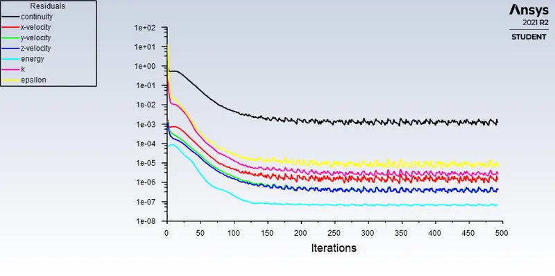
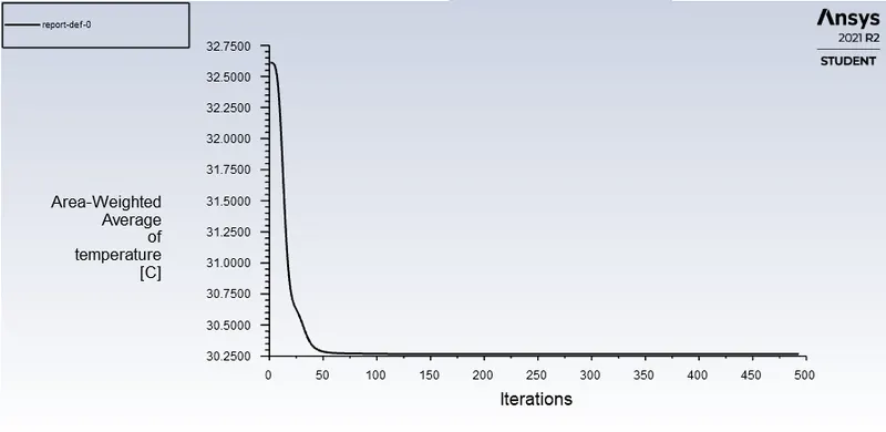
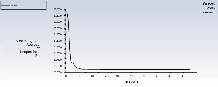
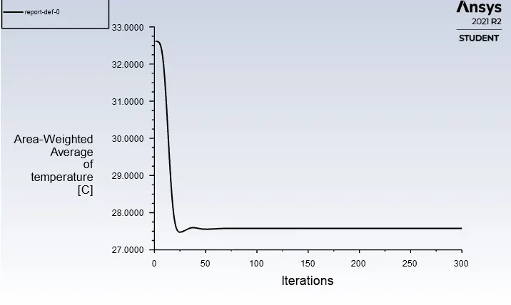
Area-Weighted Average:- This is a one type of monitor to see the average temperature in the outlet face. A weighted average helps the user gather a more accurate look at a set of data than the normal average alone. The accuracy of the numbers we arrive at with this method is determined by the weight we give specific variables in the data set. We calculate the area-weighted average on the outlet. And the specific variable is temperature.

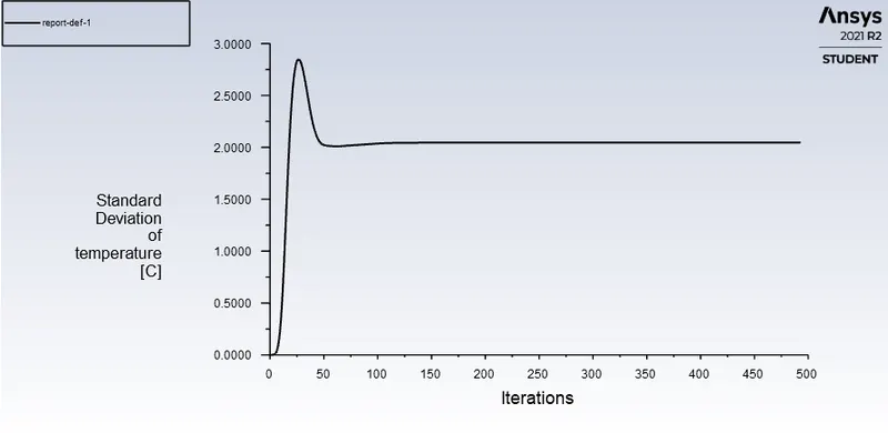
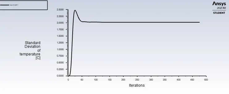
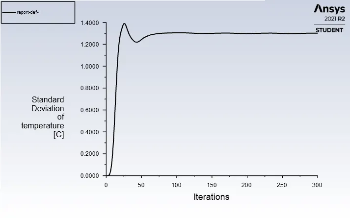
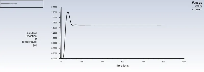
Standard Deviation :- So, here we deal with a mixing problem and in order to understand the effectiveness of mixing, the engineers look at for something that is standard deviation. Here, we calculate standard deviation of temperature of the outlet face.

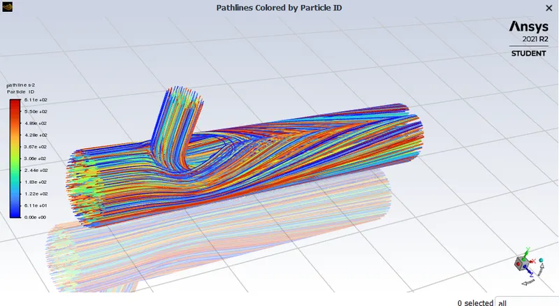
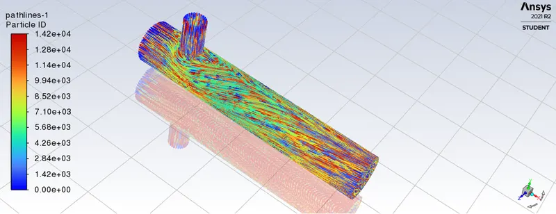
Pathlines :- This is a streamline which shows that fluid flow path.

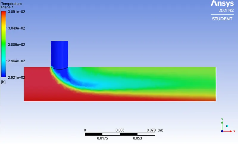
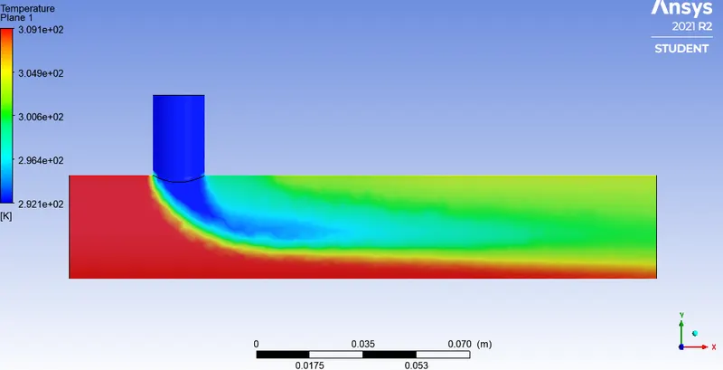
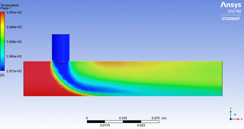
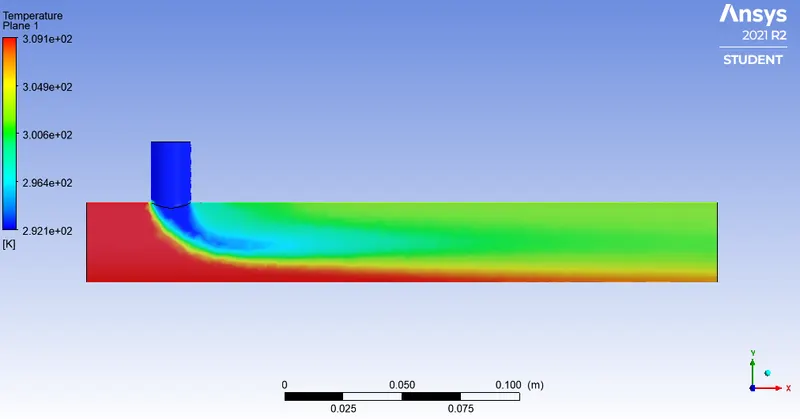
Temperature Contour:- This temperature contour plot shows that how the temperature varies in the mixing point of cold and hot fluid and over the length of the T-mixing geometry.

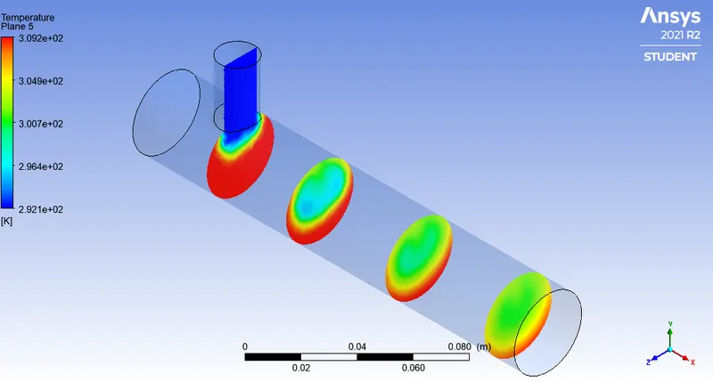
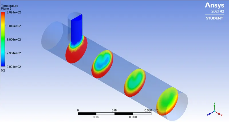
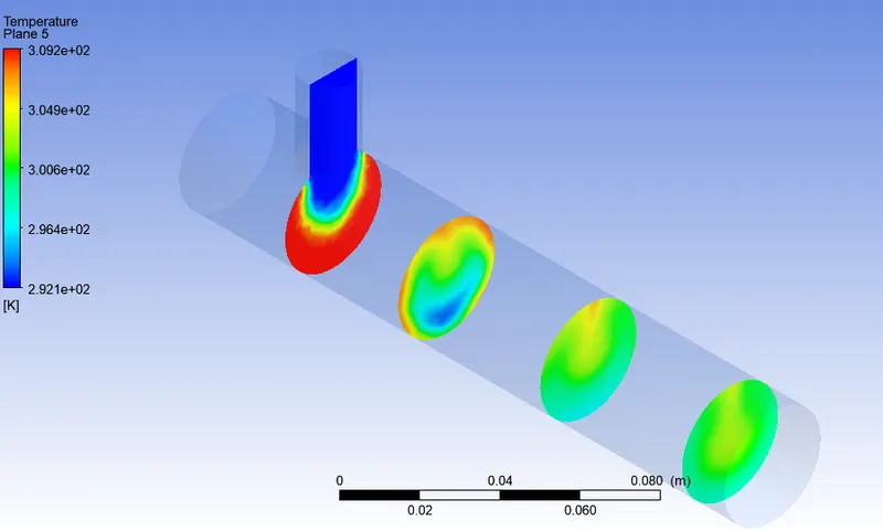
Temperature Contour:- This is also a temperature contour plot in yz plane for better visualization of mixing of two fluids in different temperature.

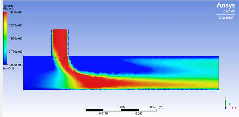
Velocity Contour:-

Line Plot:-

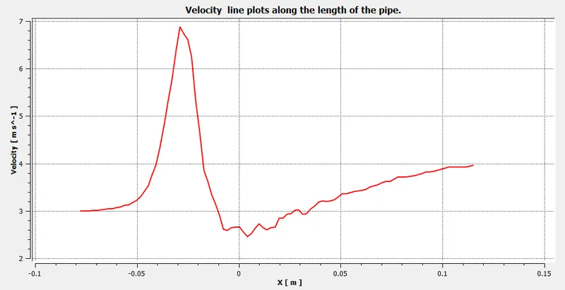
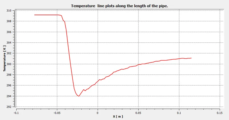
Velocity and Temperature line plots along the length of the pipe

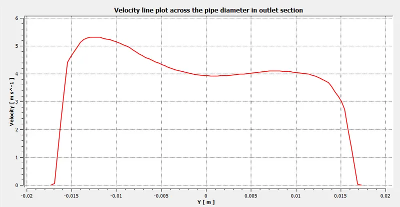
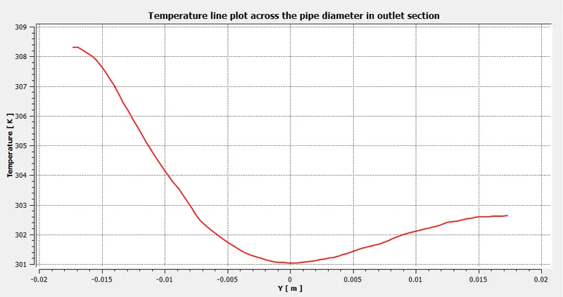
Velocity and Temperature line plots across the pipe

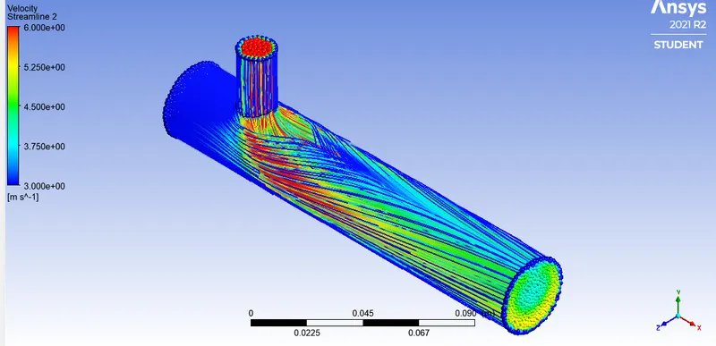
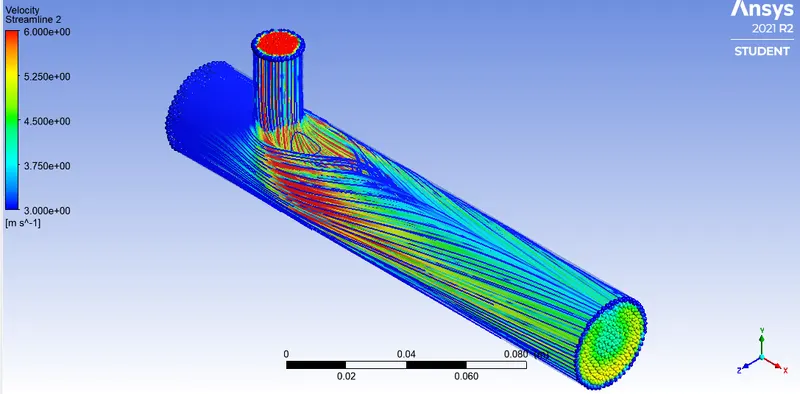
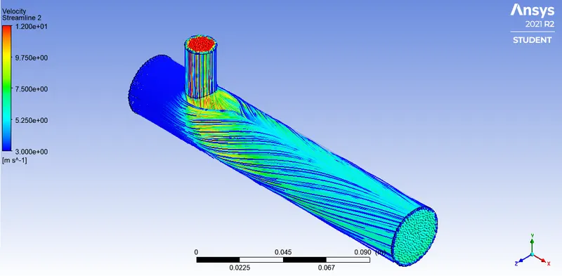
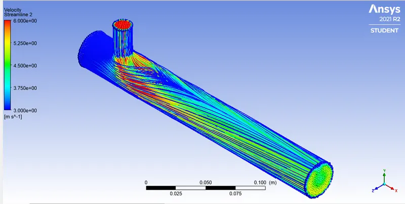
Velocity Streamline:- This is a velocity Streamline for better visualization of flow of two fluids.

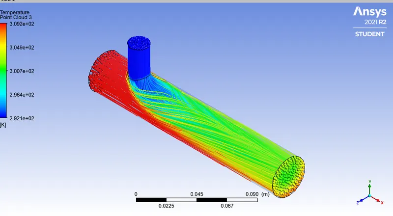
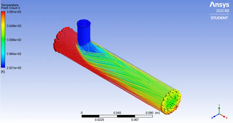
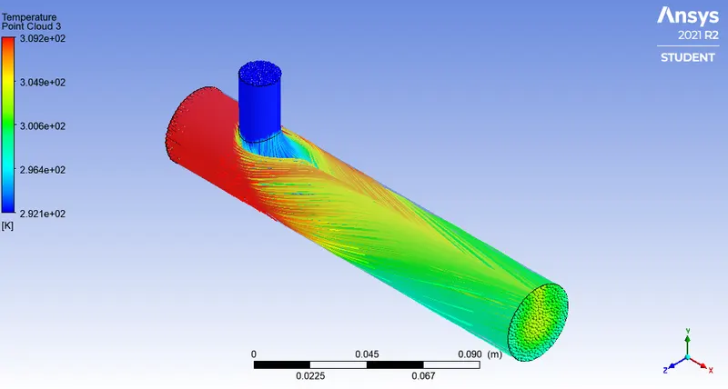
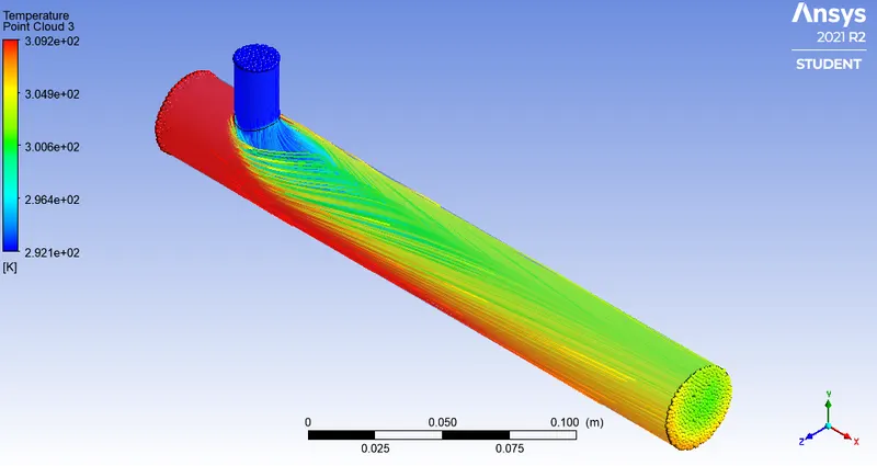
Temperature Streamline:- This is the temperature streamline for visualizing how the two fluids carries the temperature and heat exchanges between each other by mixing.

1. B)In this case, the momentum ratio is 2, which means hot inlet velocity is 3m/s and cold inlet velocity is 6m/s. And the hot inlet temperature is 36 `℃` and the cold inlet temperature is 19 `℃`. Here, we use K - Omega model for simulation:-

In this simulation, our geometry is the same as the previous geometry and the mesh is also the same as the previous. So, we only focus on our results.

RESULTS:- After settting up all the boundary and initial condition, we initialized our model using Hybrid initialization method and run the calculation. Our model is updated after each iteration.

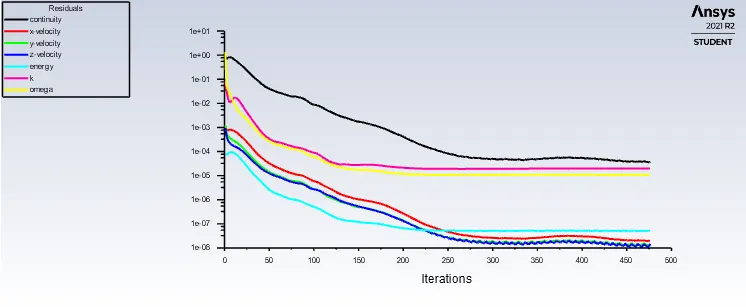
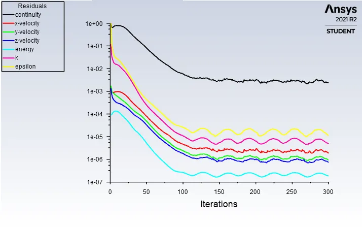
Residuals:- We previously discussed about the residuals. Here after 250 iterations all the convergence criteria are stabled.

Area-Weighted Average of Temperature:-

Standard Deviation of Temperature:-

Pathline of Fluid Flow:-

Temperature Contour Plot:-

Temperature Contour Plot2:-

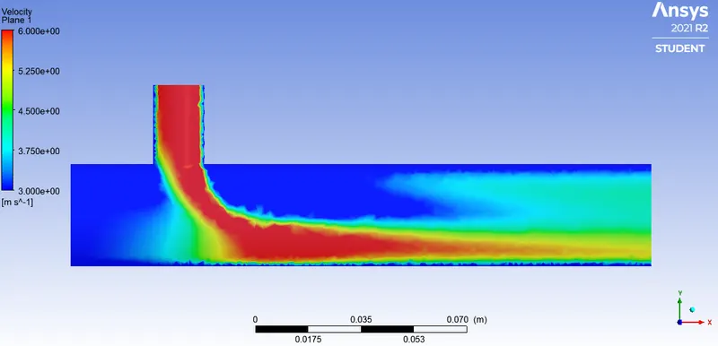
Velocity Contour:-

Line Plot:-

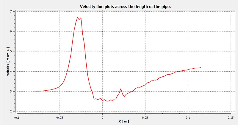
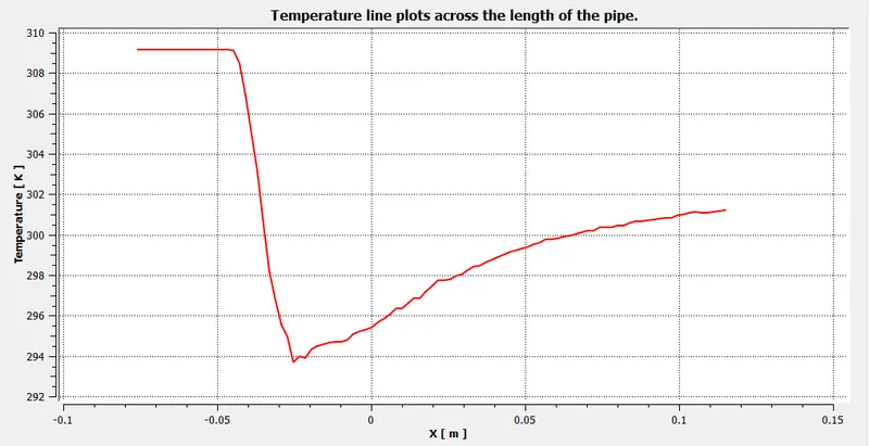
Velocity and Temperature line plots along the length of the pipe

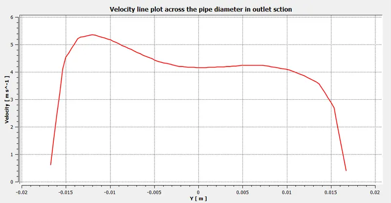
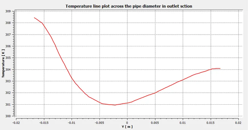
Velocity and Temperature line plots across the pipe diameter in outlet section

Velocity Streamline:-

Temperature Streamline:-

COMPARISION BETWEEN K-EPSILON MODEL AND K-OMEGA MODEL:- If we see the Residuals of both models, then one thing we notice is that the K-Epsilon model is converged after 150 iterations, but the K-Omega model is converged after 250 iterations. And since here the boundary layer is not our concern, so here we use the K-Epsilon model for our further simulation

2. In this case, the momentum ratio is 4, which means hot inlet velocity is 3m/s and cold inlet velocity is 12m/s. And the hot inlet temperature is 36`℃` and the cold inlet is 19 `℃`. Here, we use K - Epsilon model for simulation:- Because of geometry will same as the previous geometry, so our meshing process are the same, we just get difference in results. Here, hot inlet velocity is 3 m/s and cold inlet velocity is 12 m/s.

RESULTS:- After giving all initial condition and boundary condition, we initialize our model and run the calculation.

Residuals:- Here all the convergence criteria are stabled after 110 iterations.

Area-Weighted Average of Temperature:-

Standard Deviation of Temperature:-

Temperature Contour Plot1:-

Temperature Contour Plot2:-

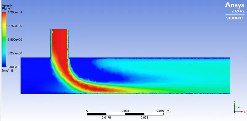
Velocity Contour:-

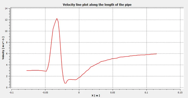
Line Plot:-

Velocity and Temperature line plots along the length of the pipe

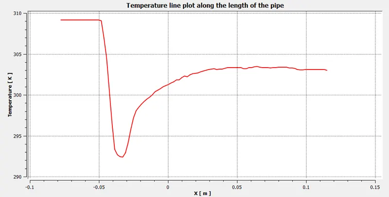
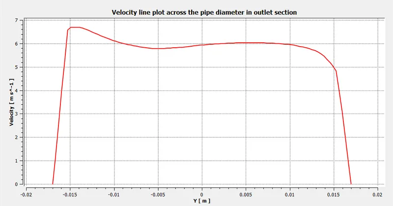
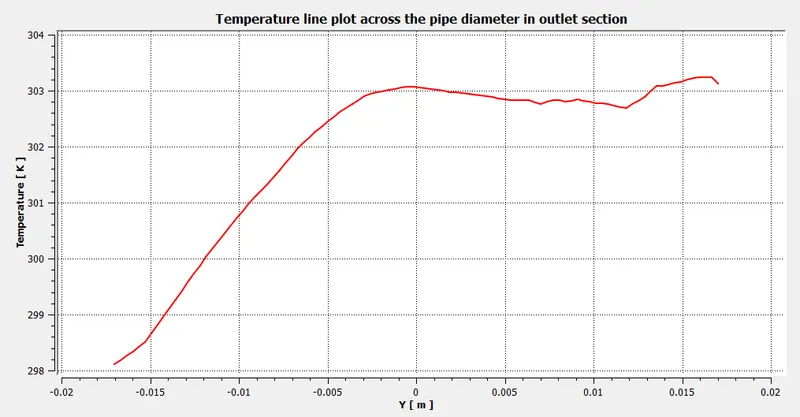
Velocity and Temperature line plots across the diameter of the pipe in outlet section

Temperature Streamline:-

Velocity Streamline:-

CASE-2:- Here we use long mixing tee for our simulation

1. In this case, the momentum ratio is 2, which means hot inlet velocity is 3m/s and cold inlet velocity is 4m/s. And the hot inlet temperature is 36`℃` and the cold inlet is 19 `℃`. Here, we use K - Epsilon model for simulation:-

For this case, we choose long mixing tee. The all processes are same as the previous simulations. We follow all the steps as mentioned in privious.

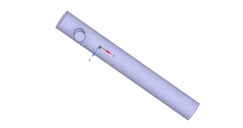
GEOMETRY:- This is a long tee geometry.

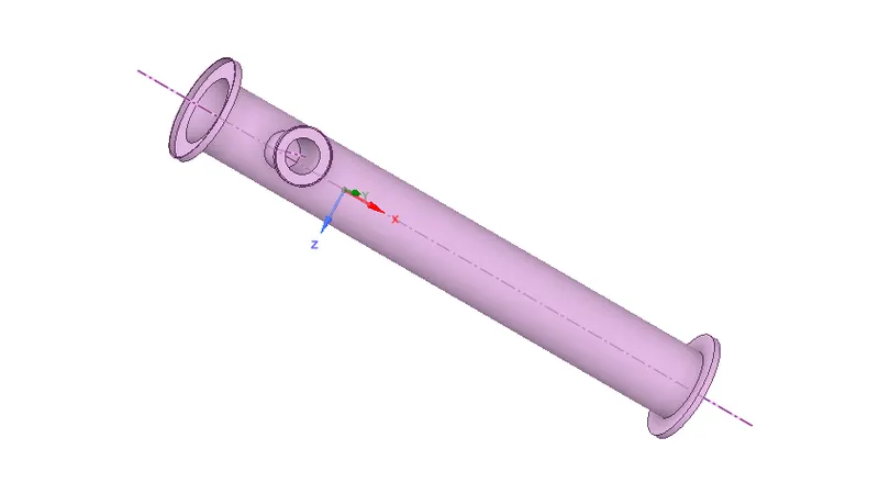
Here is the extracted volume which we get from the geometry by using Spaceclaim's beautiful features.

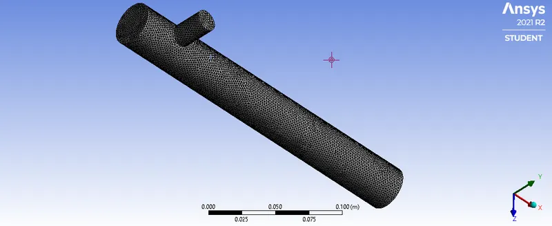
MESHING:-

This is how the mesh looks like. All the details of meshing is given below. It is a tetrahedron mesh.

This is the quality check of meshing.

This is the all details of meshing.

RESULTS:- After giving all initial condition and boundary condition, we initialize our model and run the calculation.

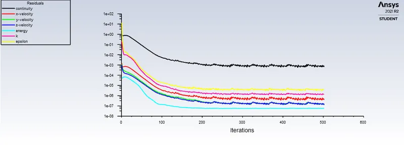
Residuals:- After 202 iterations, solutions are converged.

z

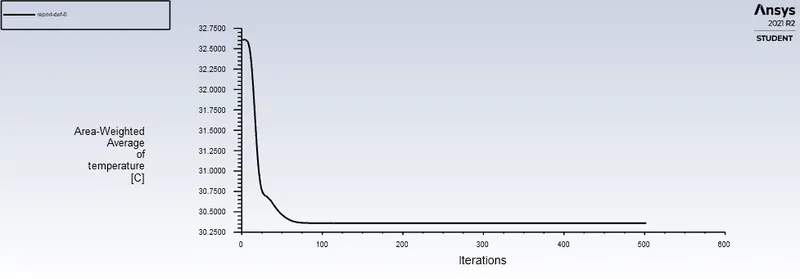
Area-Weighted Average of Temperature:-

Standard Deviation of Temperature:-

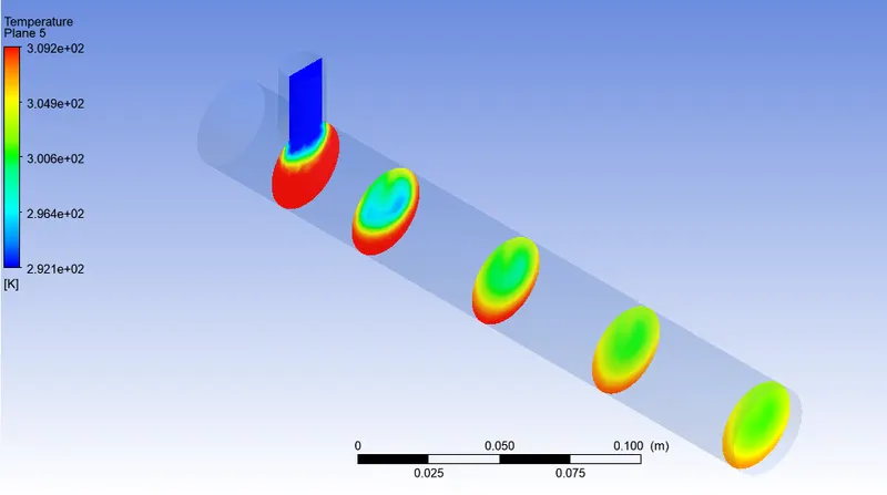
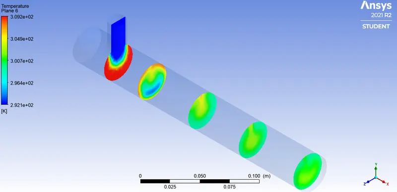
Temperature Contour Plot1:-

Temperature Contour Plot2:- This is a

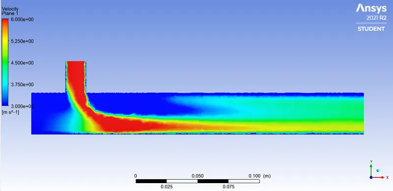
Velocity Contour Plot:-

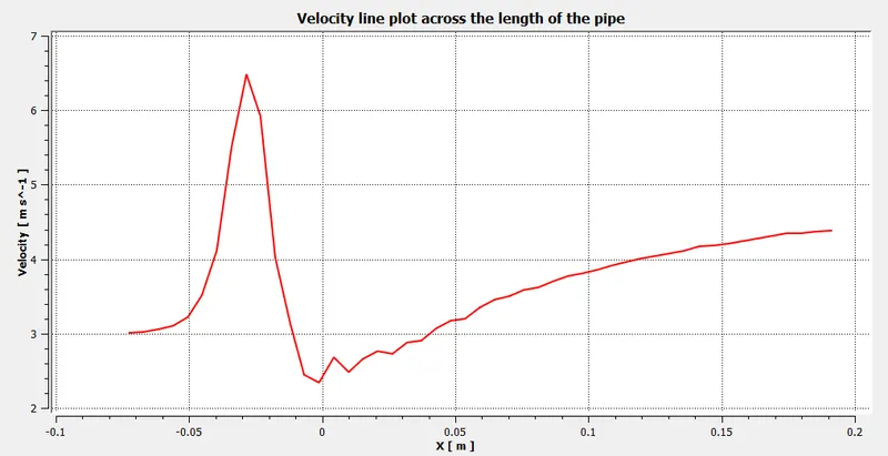
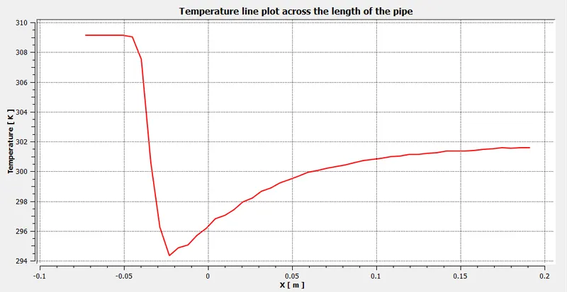
Line Plot:-

Velocity and Temperature line plots along the length of the pipe

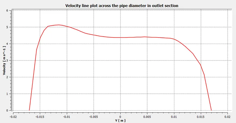
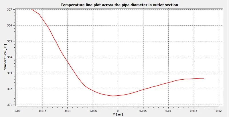
Velocity and Temperature line plots across the diameter of the pipe in outlet section

Temperature Streamline:-

Velocity Streamline:-

2. In this case, the momentum ratio is 4, which means hot inlet velocity is 3m/s and cold inlet velocity is 12m/s. And the hot inlet temperature is 36`℃` and the cold inlet is 19 `℃`. Here, we use K - Epsilon model for simulation:-

This is a part of case2 and the geometry and meshing are the same as in the previous simulation. The only difference is that the momentum ratio. Here the momentum ratio is 4, which means hot inlet velocity is 3 m/s and cold inlet velocity is 12 m/s.So we don't again go for the geometry extraction and meshing process, here we just focus on the results.

RESULTS:- After giving all initial condition and boundary condition, we initialize our model and run the calculation.

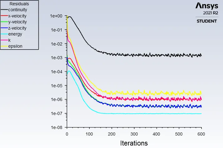
Residuals:- After 150 iterations, solutions are converged.

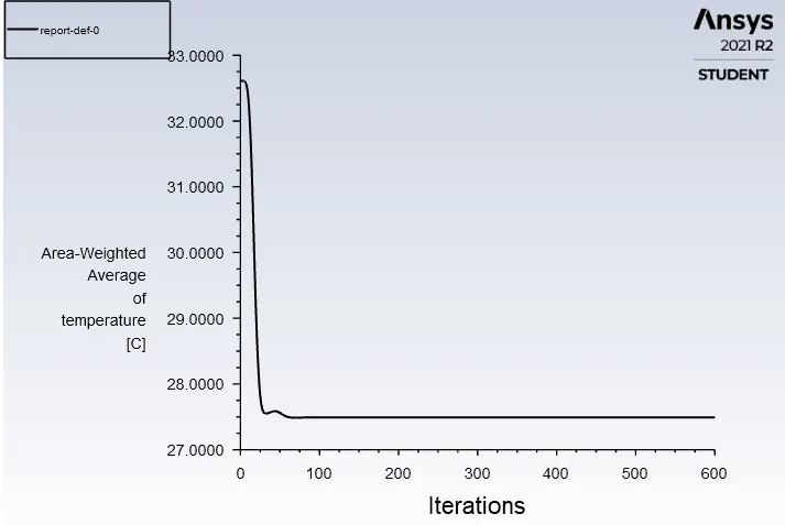
Area-Weighted Average of Temperature:-

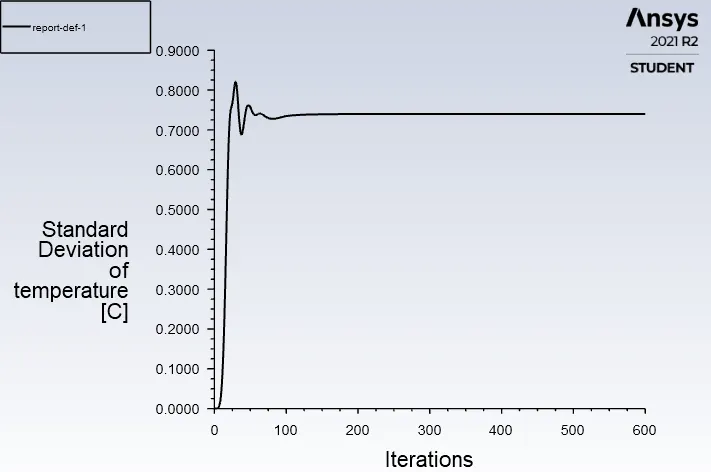
Standard Deviation of Temperature:-

Temperature Contour Plot1:-

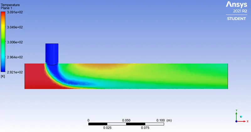
Temperature Contour Plot2:-

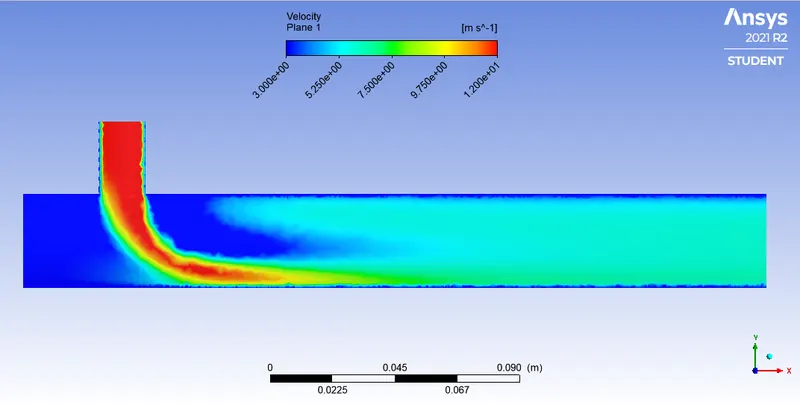
Velocity Contour:-

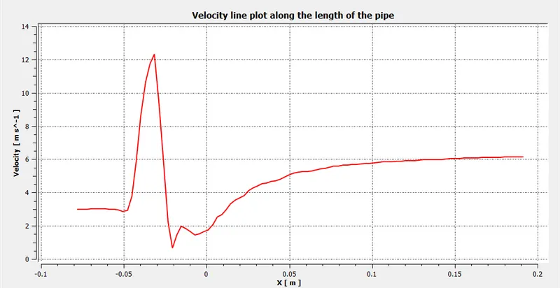
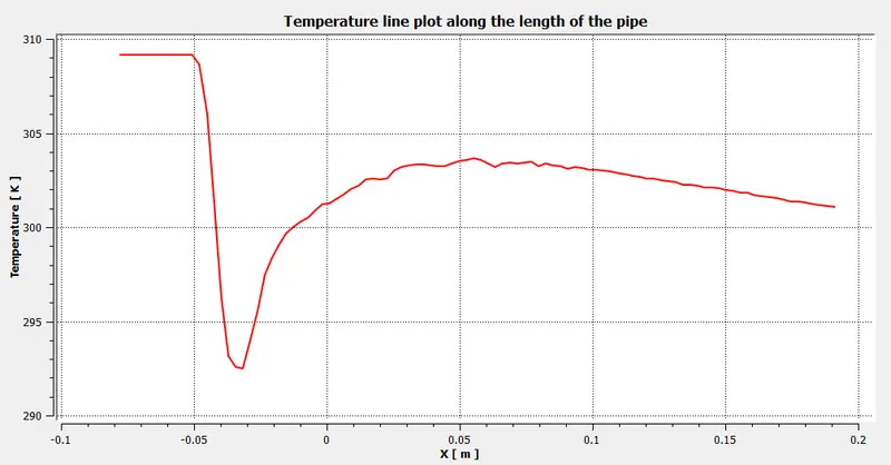
Line Plot:-

Velocity and Temperature line plots along the length of the pipe

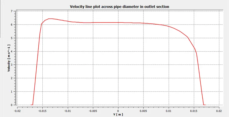
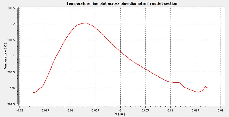
Velocity and Temperature line plots across the diameter of the pipe in outlet section

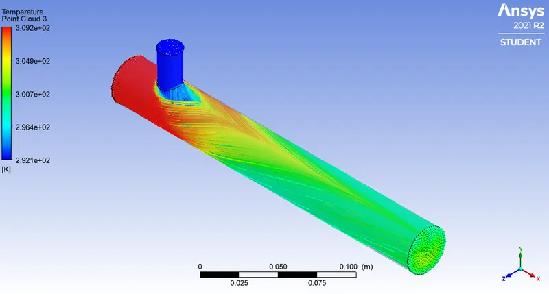
Temperature Streamline:-

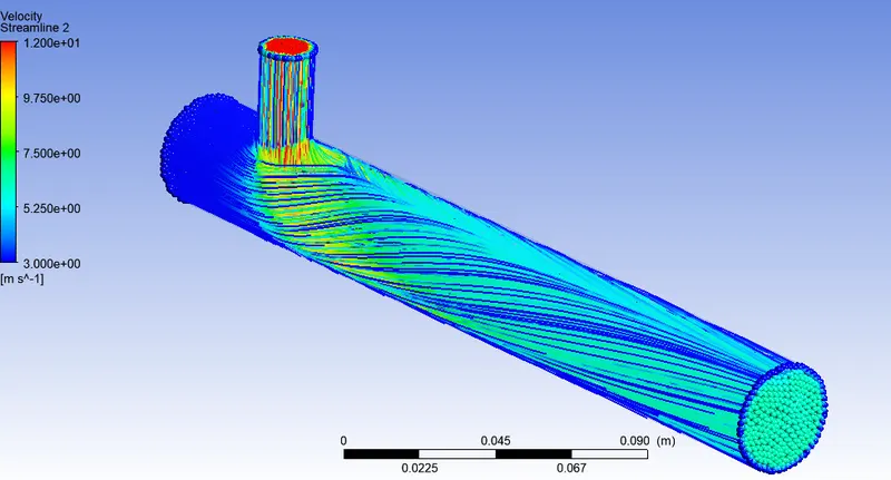
Velocity Streamline:-

OBSERVATION:- Here we do 5 simulations but we discussed only 4 which simulations we do use the k-epsilon model. And why we choose the k-epsilon model we discuss in the previous section. we discussed what we see in the simulation one by one.

1. In the first simulation for case_1, we use a short mixing tee and the momentum ratio is 2. We see hereafter 150 iterations the solution is converged. But two fluids are not mixed properly. If we see the line plot of temperature along the length of the pipe, there we see 309k means 36 ℃ continuously goes till the mixing has not occurred and in the mixing position the temperature suddenly drops in 292k or 19℃ and then after mixing it goes up and the last temperature is 302.5k. If we see the line plot the temperature across the pipe in the outlet section, the temperature varies between 309k to 301k. So this is not acceptable. And if we see the velocity line plot across the pipe in the outlet section, we can observe there is a curve that starts from zero and end in zero. This is nothing but boundary condition, when the air is in contact with the pipe wall there we see no sleep boundary condition means their air velocity is zero. And the air velocity is increasing towards the center of the pipe.
2. In the second simulation for case_1, we use a short mixing tee and the momentum ratio is 4. We see hereafter 110 iterations the solution is converged. If we see the line plot of temperature along the length of the pipe, there we see 309k means 36 ℃ continuously goes till the mixing does not occur and in the mixing position the temperature suddenly drops in 292k or 19℃ and then after mixing it slowly rises and the last temperature is 303k. If we see the line plot the temperature across the pipe in the outlet section, the temperature varies between 304k to 298k means 31 ℃ to 25 ℃. So, we can say the mixing is quite good and the two fluids are transferring heat to each other very goodly.
3. In the third simulation for case_2, we use a long mixing tee and the momentum ratio is 2. We see hereafter 202 iterations the solution is converged. If we see the line plot of temperature along the length of the pipe, there we see 309k means 36 ℃ continuously goes till the mixing has not occurred and in the mixing position the temperature suddenly drops in 294k or 21 ℃ and then after mixing it slowly goes up and the last temperature is 301.8k. If we see the line plot the temperature across the pipe in the outlet section, the temperature varies between 307k to 301k. So, here also we can say the mixing is quite good and the two fluids are transferring heat to each other very goodly.
4. In the fourth simulation for case_2, we use a long mixing tee and the momentum ratio is 4. We see hereafter 160 iterations the solution is converged. If we see the line plot of temperature along the length of the pipe, there we see 309k means 36 ℃ continuously goes till the mixing has not occurred and in the mixing position the temperature suddenly drops in 292k or 19 ℃ and then after mixing it slowly goes up and the last temperature is 301k. If we see the line plot the temperature across the pipe in the outlet section, the temperature varies between 302.5k to 299.5k. So, here we see how beautifully the two fluids are mixing and transferring heat with each other.

Observation Table

Cell count	Average outlet temperature	Number of iterations for convergence
104716	305K(309K to 301K)	150
104716	301K(304K to 298K)	110
140244	304K(307K to 301K)	202
140244	301K(302.5K to 299.5K)	160

CONCLUSION:- Now we can conclude that in the fourth simulation where we choose a long mixing tee and the momentum ratio is 4, that mixing is best from any other mixing. There mixing is so beautifully happened, that we see a very small temperature difference in our outlet section.