Week 1- Mixing Tee
Question
For this challenge, we have created two versions of the mixing tee. One of them is longer than the other.
Your job is to set up steady-state simulations to compare the mixing effectiveness when hot inlet temperature is 360C & the Cold inlet is at 190C.
Use the k-epsilon and k-omega SST model for the first case and based on your judgment use the more suitable model for further cases. Giving the reason for choosing a suitable model is compulsory.
- Case 1
- Short mixing tee with a hot inlet velocity of 3m/s.
- Momentum ratio of 2, 4.
- Case 2
- Long mixing tee with a hot inlet velocity of 3m/s.
- Momentum ratio of 2, 4.
**Momentum ratio = velocity at cold inlet / velocity at hot inlet**
Answer
The use of a mixing tee is to mix well two different fluids, or fluids of two different temperatures. The design of a mixing tee is such that two pipes of different diameters are joined in 90 degrees or like a T- shape, therefore the name. A good mixing can be achieved by either increasing the length of the tube or increasing the inlet velocity.
The two viscous models asked here are
k-epsilon
The k-epsilon model is the most common model used in CFD to simulate mean flow characteristics for turbulent model conditions. It is a two-equation model that gives a general description of turbulence by means of two PDE. The original impetus for the K-epsilon model was to improve the mixing-length model, as well as to find an alternative to algebraically prescribing turbulent length scales in moderate to high complexity flows.
K-omega
In CFD, the k–omega turbulence model is a common two-equation turbulence model, that is used as an approximation for the Reynolds-averaged Navier–Stokes equations (RANS equations). The model attempts to predict turbulence by two partial differential equations for two variables, k and omega(w) with the first variable being the turbulence kinetic energy (k) while the second (w) is the specific rate of dissipation (of the turbulence kinetic energy k into internal thermal energy).
k-omega model of turbulence is capable of solving turbulence parameters very close to boundary or wall region. If you are interested to capture the phenomenon in such a region, you have to have very fine meshing near to the wall, so that the Y+ value should be as small as possible. on the other hand k- epsilon provides standard results. Hence we prefer k-omega as the turbulence model.
*****************************************CASE 1******************************************
FOR SHORT MIXING TEE
Shape (Geometry)
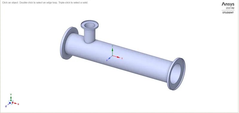
This is the mixing tee that we are going to simulate in this problem.
For the first, we need to extract the fluid volume from it, which means to extract a volume that affects the fluid flow only.
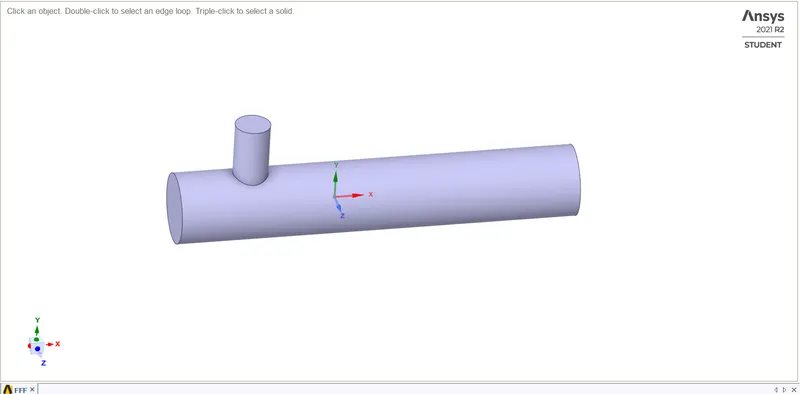
This is how extracted volume looks like.
Now, the next step is to Mesh the geometry.
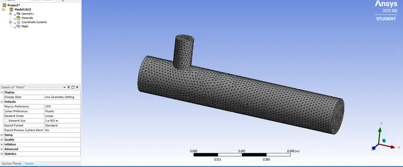
A suitable mesh size of 3 mm is used and the mesh looks cleaner. On checking the quality of the mesh, we found that the mesh is of good quality, which is more than 43%. The minimum quality needed is 5%. Hence the quality is absolutely fine.

now the next step is to assign names to the walls or faces, by using the option creating named selection.
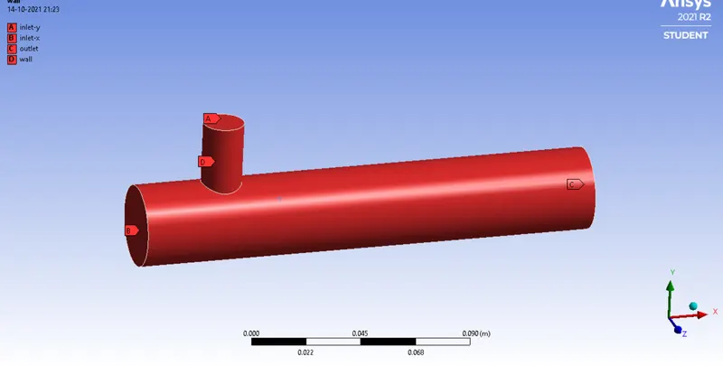
For Short Mixing Tee
Momentum ratio = 2 with the K-epsilon model.
Boundary conditions
inlet-x
Velocity- 3m/s
Temperature - 36 degrees C
inlet-y
Velocity - 6m/s
Temperature - 19 degrees C
Outlet
Guage pressure = 0 pascal
Total number of iterations = 400
Results
Area-Weighted average of Temperature
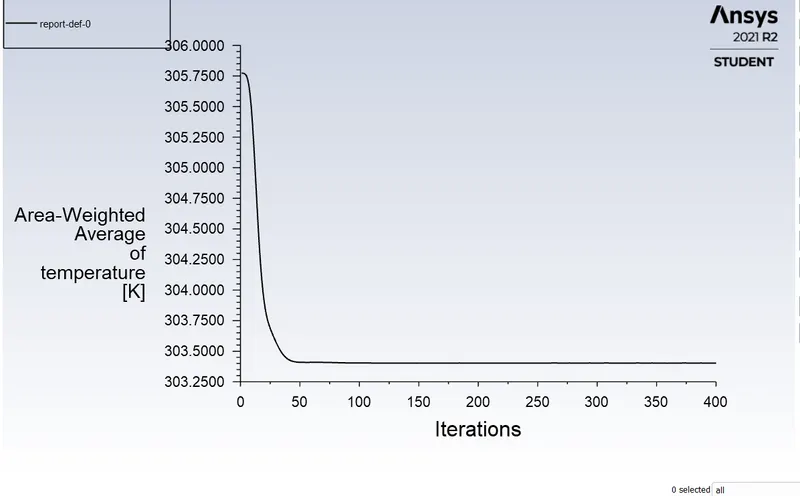
Area weighted average of temperature = 303.3 K
Standard Deviation of Temperature
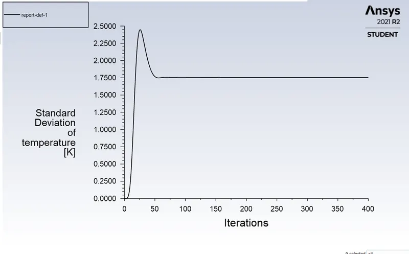
The standard deviation of temperature is 2.4500 K
Convergence Residual Plot
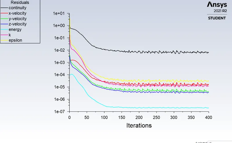
Number of Iterations to converge = 150
Graphical Representation of Results
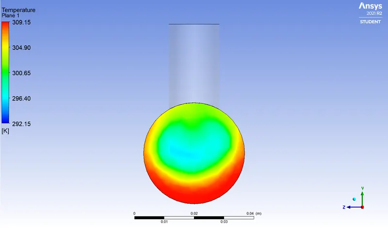
Temperature Contour along the length of the pipe
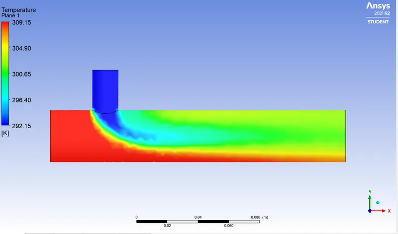
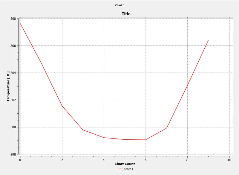
Line chart of Temperature across the length of the pipe
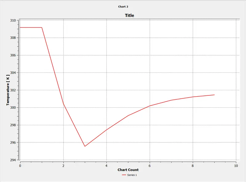
Temperature contour along the Cut plane
Line chart of Temperature across the cross sectional
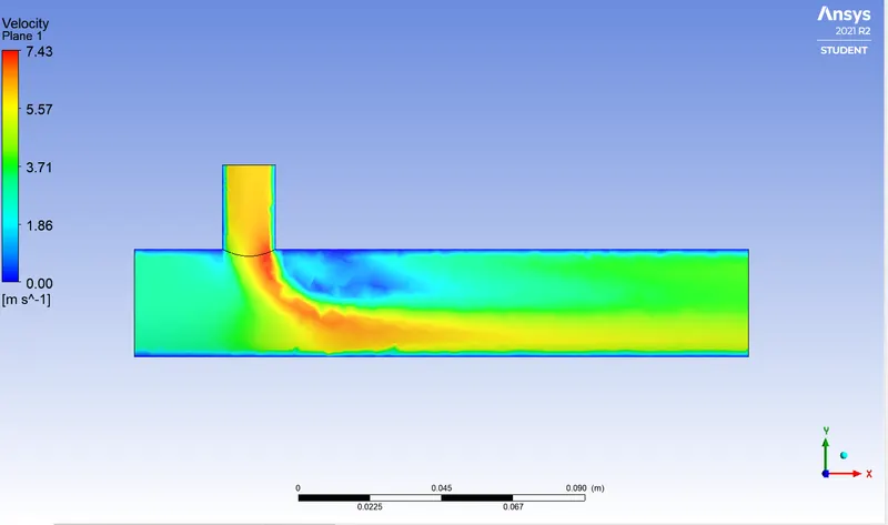
velocity contour along the length of the pipe.
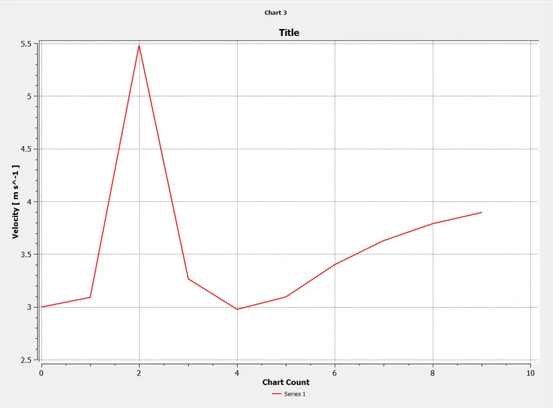
Line chart of velocity across the length of the pipe
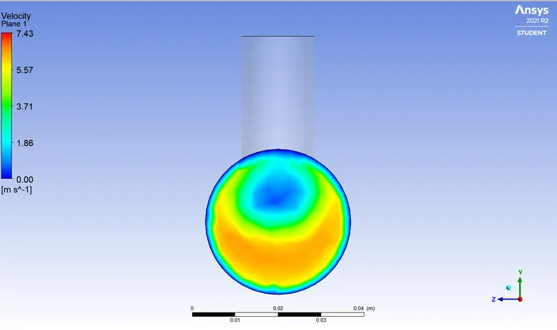
Velocity contour along the cut plane
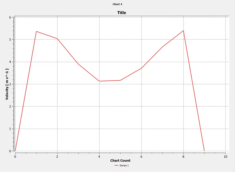
Line chart of velocity across the cross sectional area
************************************Case 1.1**********************************************
For Short Mixing Tee
Momentum Ratio = 4 with K-epsilon model
Boundary Condition
Inlet-x
Velocity - 3m/s
Temperature - 36*C
Inlet -y
Velocity - 12m/s
Temperature - 19*C
Outlet
Guage pressure = 0 pascal
Results
Standard Deviation
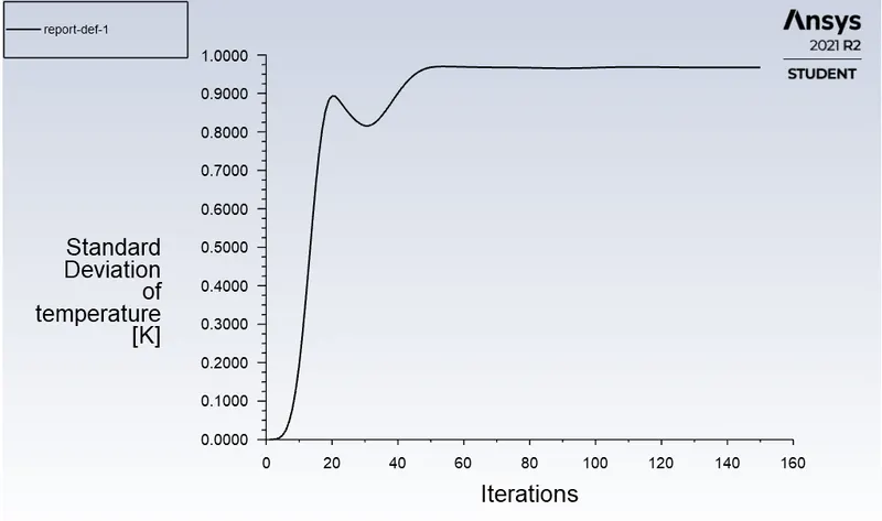
The standard Deviation temperature is 0.98K
Area-Weighted Average Temperature
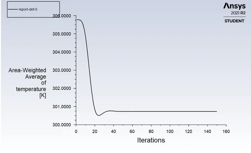
An area-Weighted average temperature is 300.05K
Residual
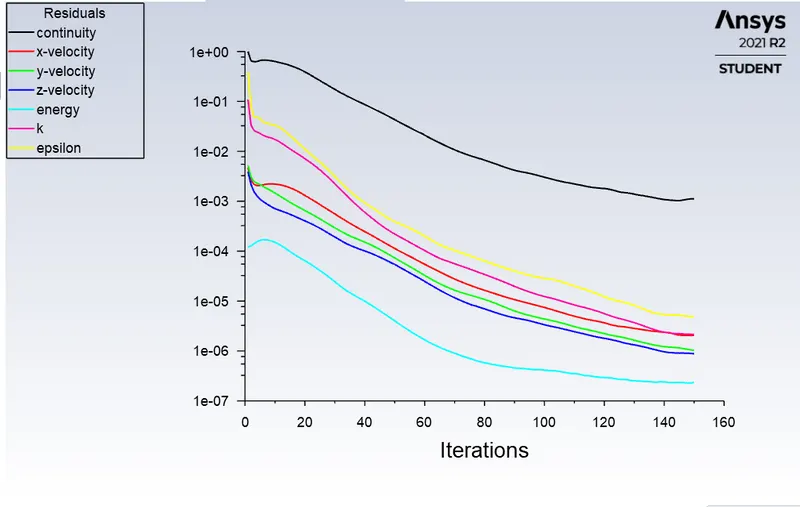
Graphical Representation
Temperature along the length of the pipe
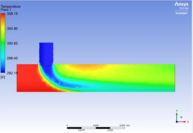
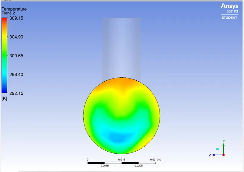
Temperature along the cross section
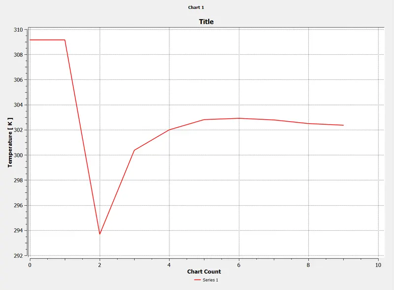
Line graph of Temperature along the length of the pipe
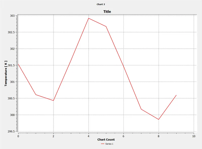
Temperature along the Cross-section of the pipe
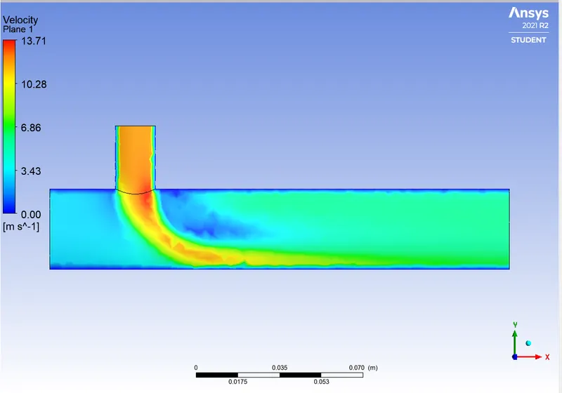
Velocity along the length of the pipe.
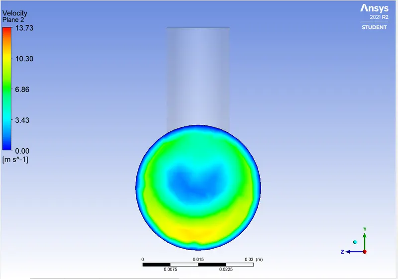
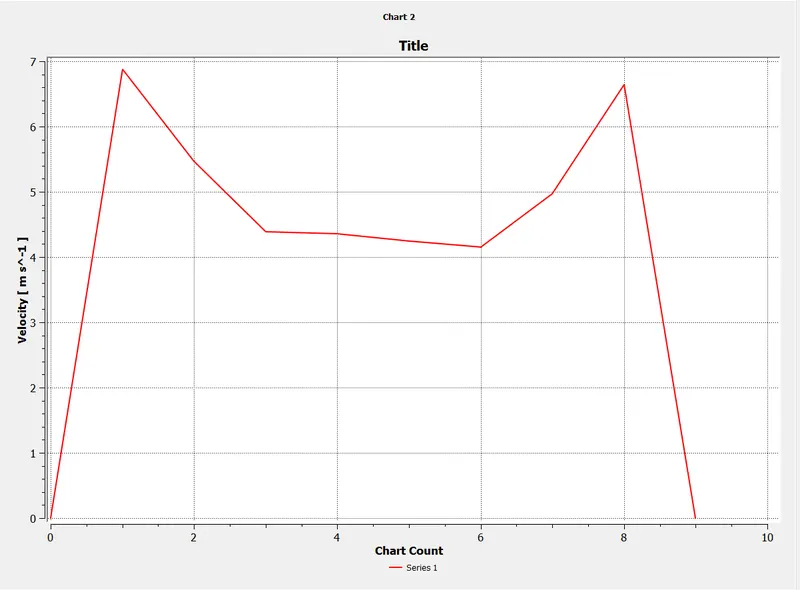
Velocity along the cross section of the pipe
Line chart o f velocity along the length of the pipe
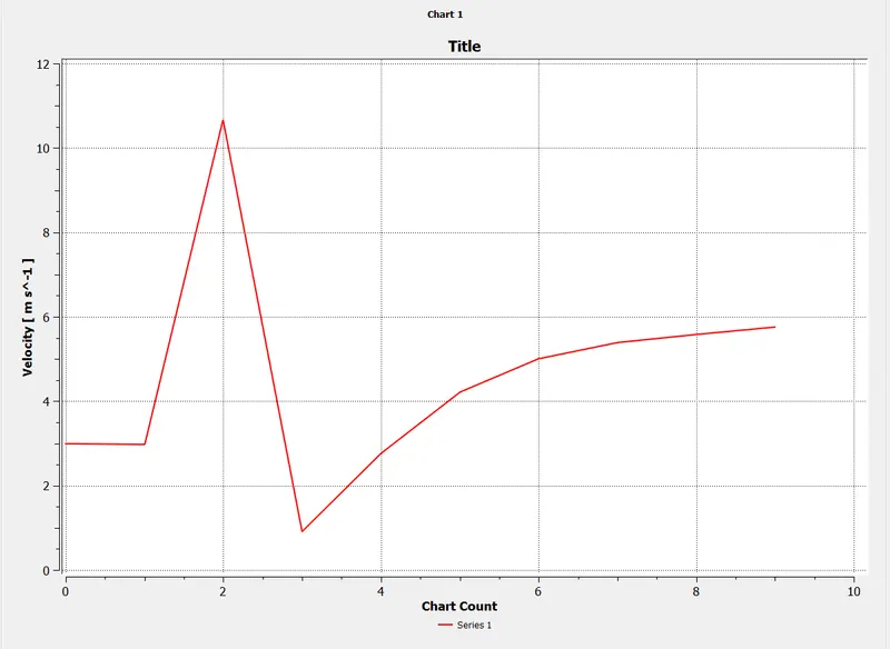
Line chart of Velocity along the cross section of the pipe
****************************************CASE 1.2*****************************************
For Momentum ratio = 2
Turbulence Model = K omega
Boundary Conditions
Inlet-x
Velocity = 3m/s
Temperature = 36*C
Inlet-y
Velocity = 6m/s
Temperature = 19*C
Outlet
Guage Pressure = 0 pascal
Results
Area-Weighted average of Temperature
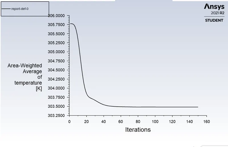
Area - Weighted average of Temperature = 303.400 K
Standard Deviation of Temperature
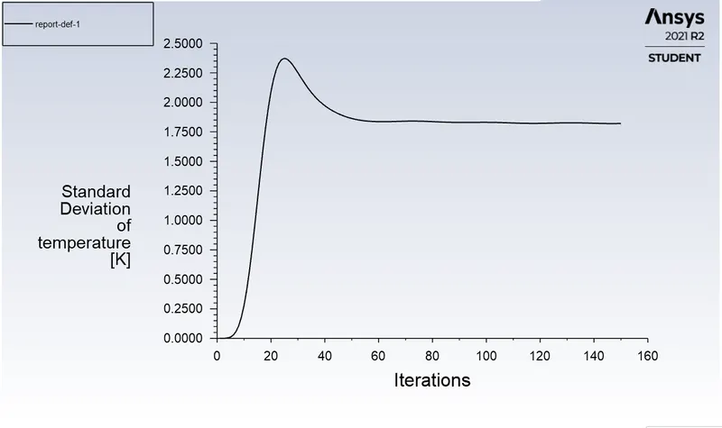
Standard Deviation of Temperature = 1.800 K
Residuals
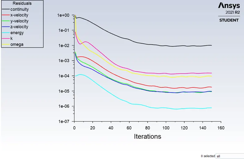
Graphical Representations
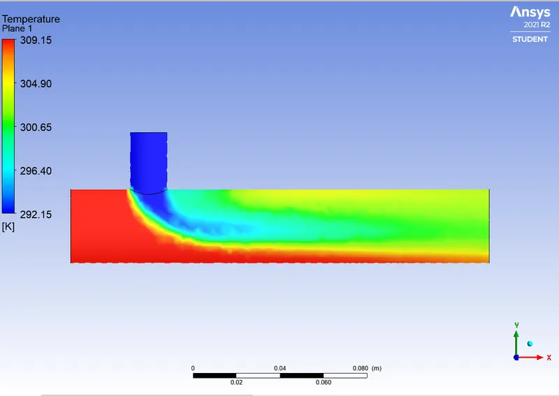
Temperature contour along the length of the pipe
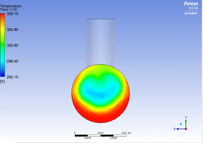
Temperature contour along the CS
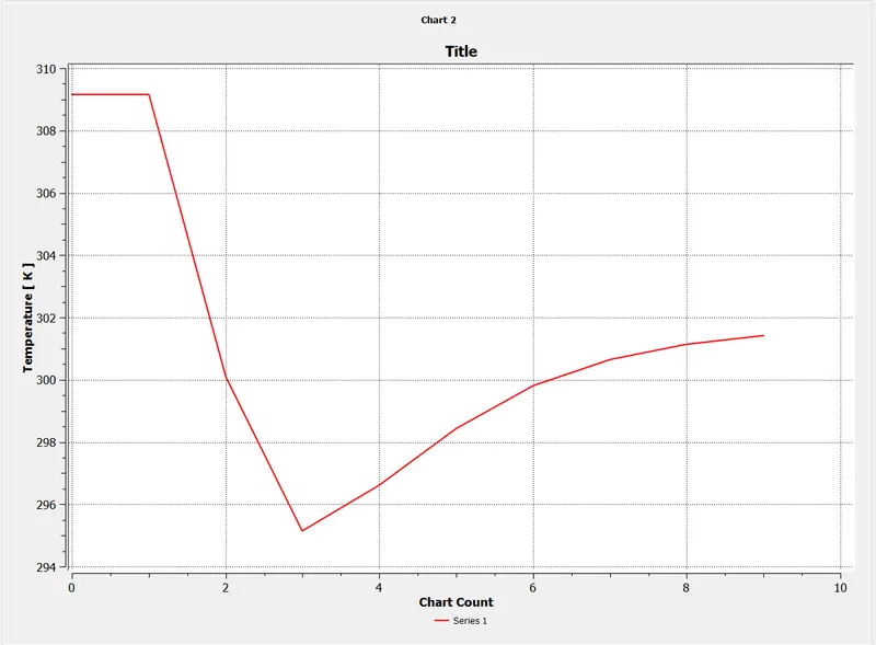
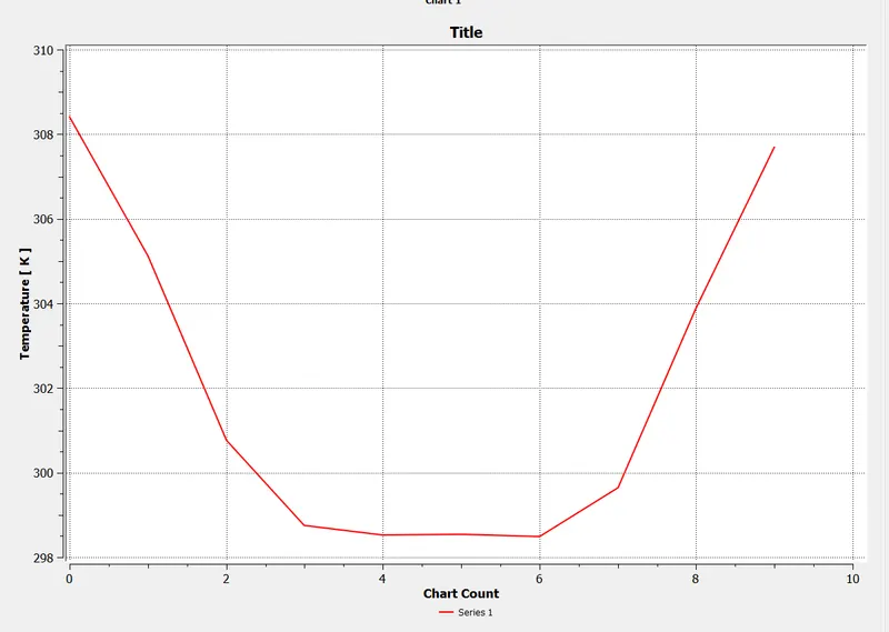
Line chart of temp along the length of the pipe
Line chart of temperature along the CS
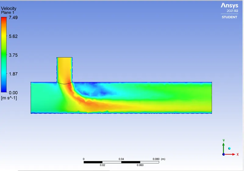
Velocity contour along the length of the pipe
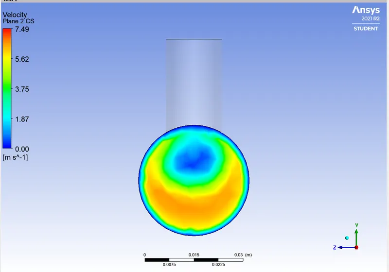
Velocity Contor along the CS of the pipe
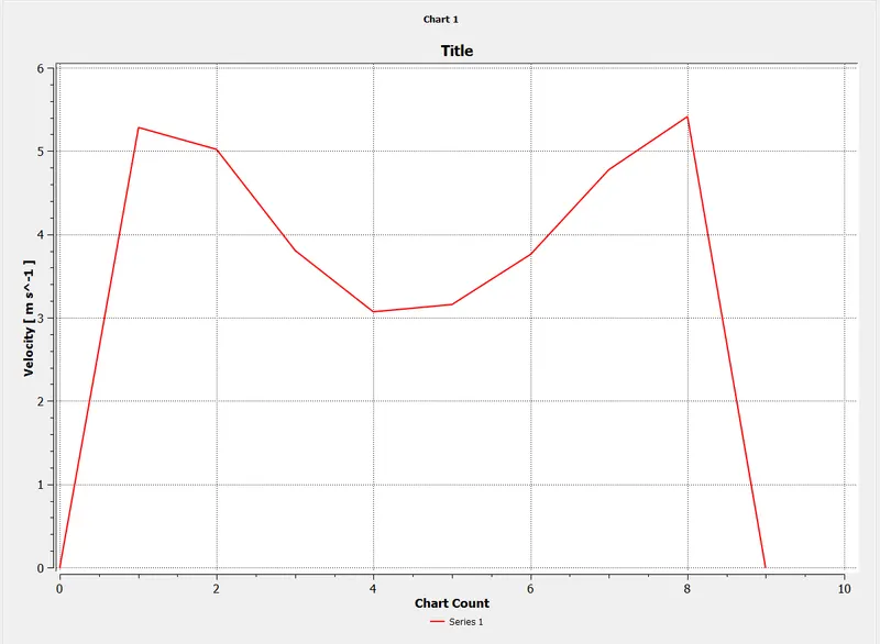
Line chart of Velocity along the length of the pipe
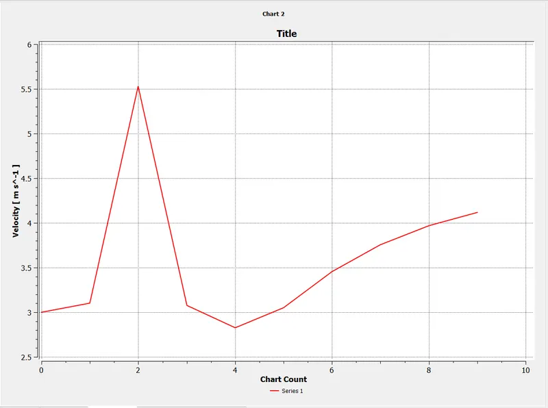
Line Chart of Velocity along the Cross section
************************************CASE 1.3*********************************************
Momentum Ratio = 4
Turbulence model = K omega
Boundry Condition
inlet -x
Velocity = 3m/s
Temperature = 36*C
Inlet-y
Velocity = 12 m/s
Temperature = 19*C
Outlet
Guage pressure = 0 pascal
Results
Area- Weighted average of temperature
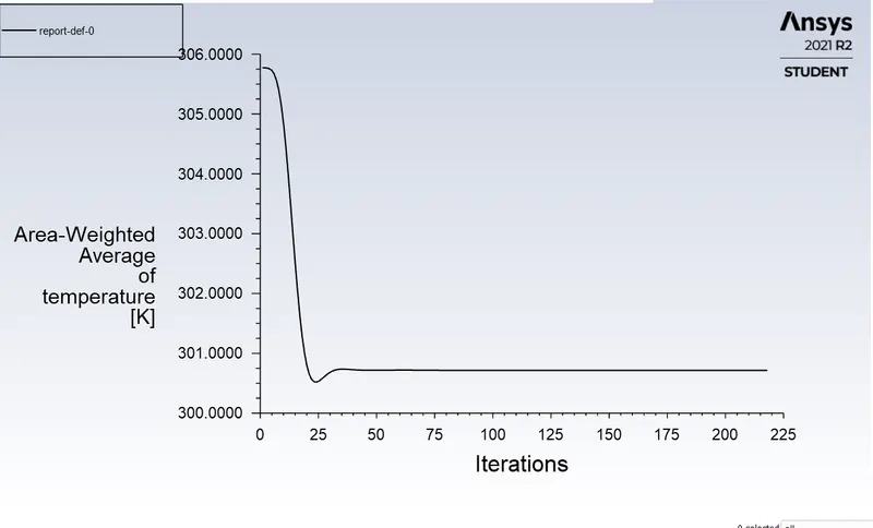
Area- Weighted average of temperature = 300.500
Standard Deviation of Temperature
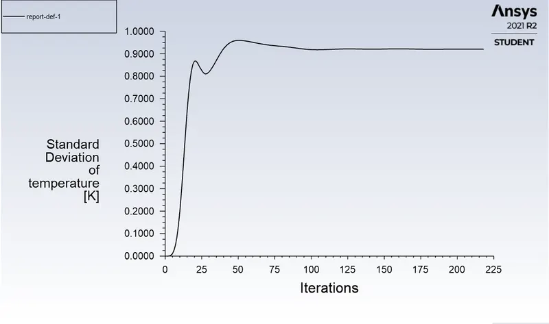
Standard Deviation of Temperature = 0.9500K
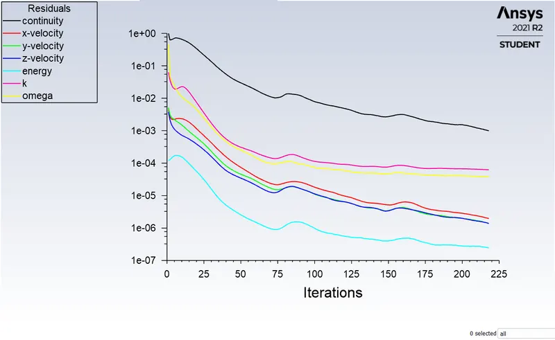
Residuals
Graphical Representation of Results
Temperature contour along the length of the pipe
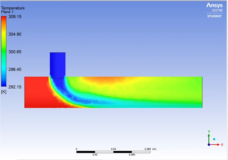
Temperature along the Cross section
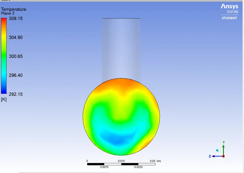
Line chart of temperature along the length of the pipe
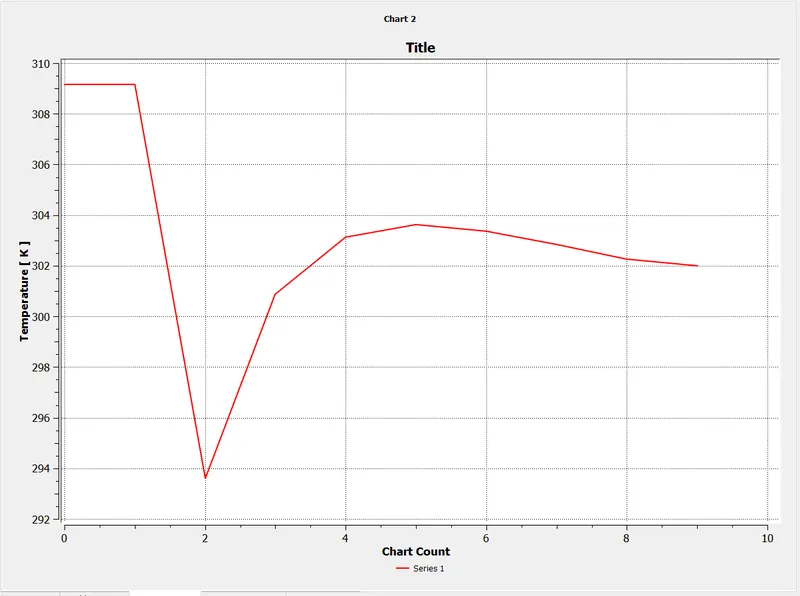
Temperature along the Cross section
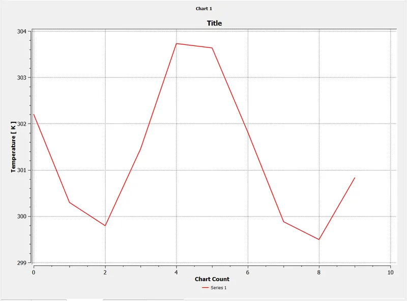
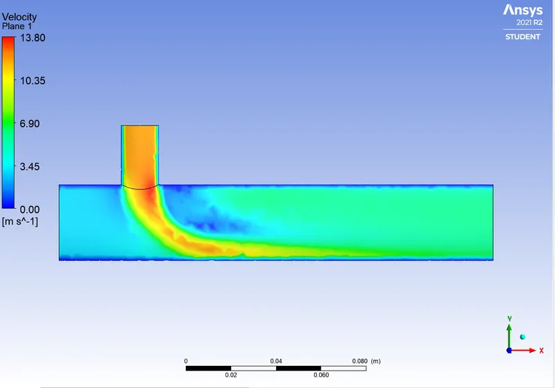
Velocity contour along the length of the pipe
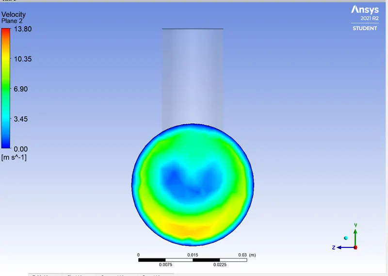
Velocity contour along the Cross section of the pipe
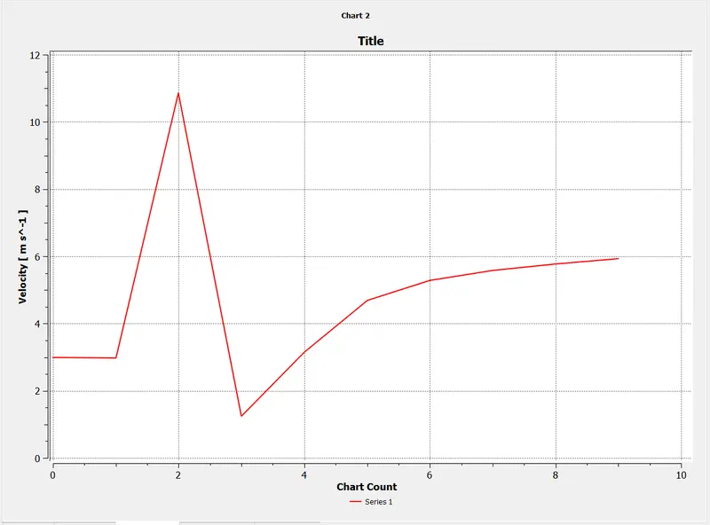
Line Chart of Velocity along the length of the pipe
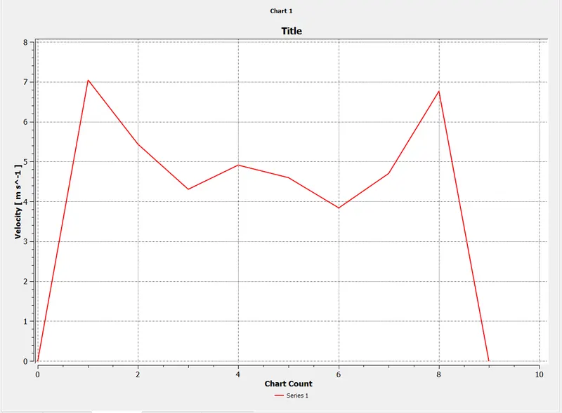
line chart of velocity along the cross section of the pipe
****************************************CASE 2*******************************************
FOR LONG MIXING TEE
Geometry creation
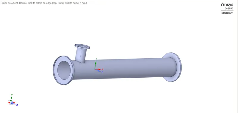
The volume for the fluid flow is extracted from the geometry
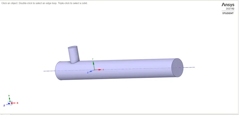
after volume extraction a meshing with element size of 3mm is done.
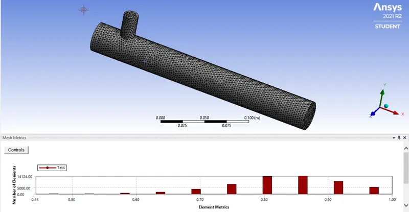
from the above table its clear that the quality of the mesh is good , that is above 44%.
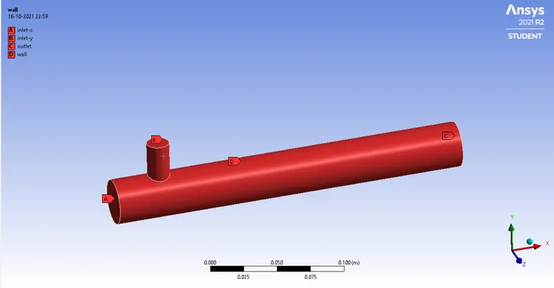
now, we create named selection for every walls
CASE 2.1
For Momentum Ratio = 2
Boundary Conditions
Inlet-x
Velocity = 3m/s
Temperature = 36*C
Inlet -y
velocity= 6m/s
Temperature = 19*C
Outlet
Guage pressure = 0 pascal
Results
An area-Weighted average of temperature
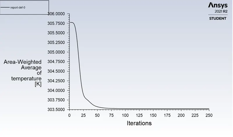
Temperature is = 303.6 K
Standard Deviation of Temperature
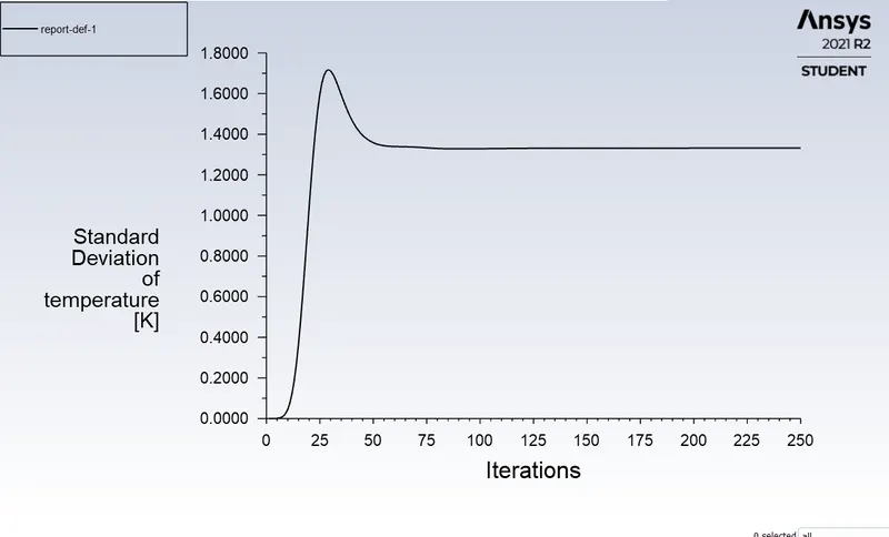
Temperature is 1.72 K
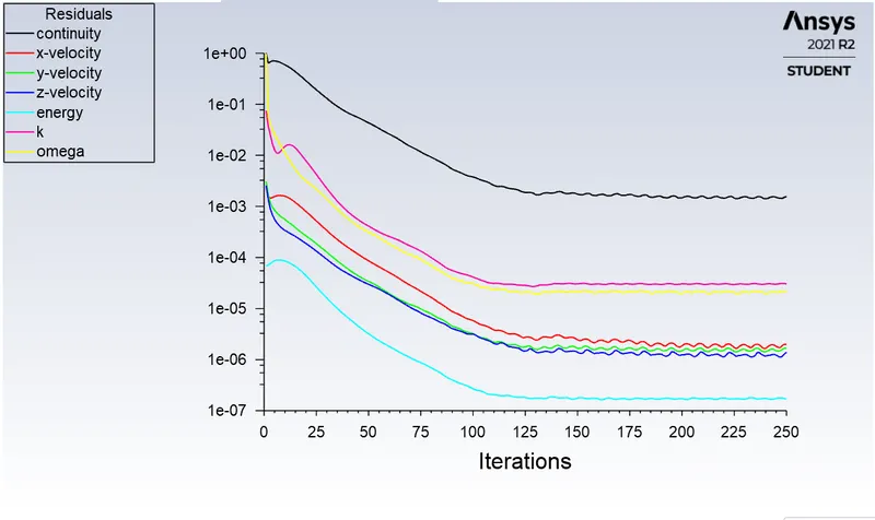
Residuals
Graphical Representations of Results
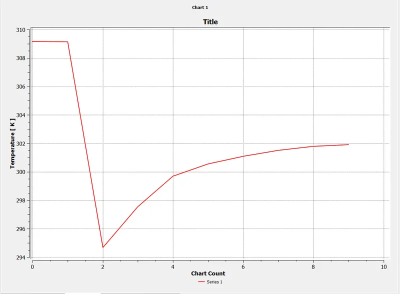
Temperature along the length of the pipe
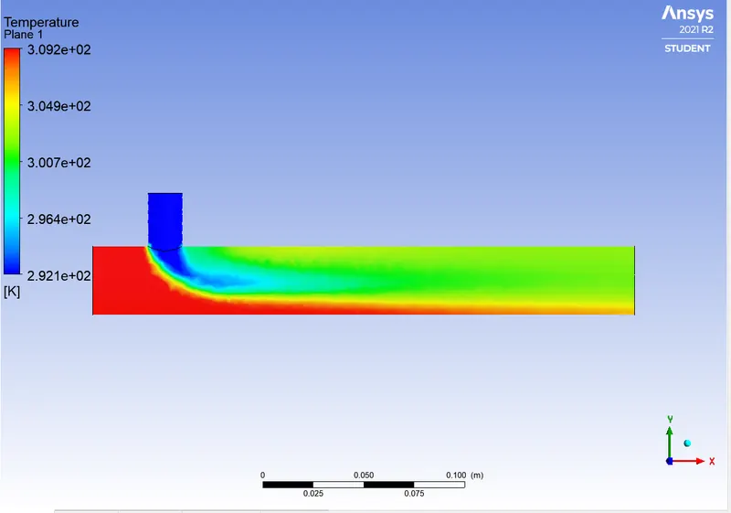
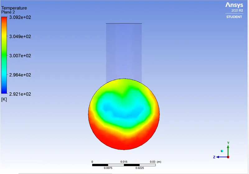
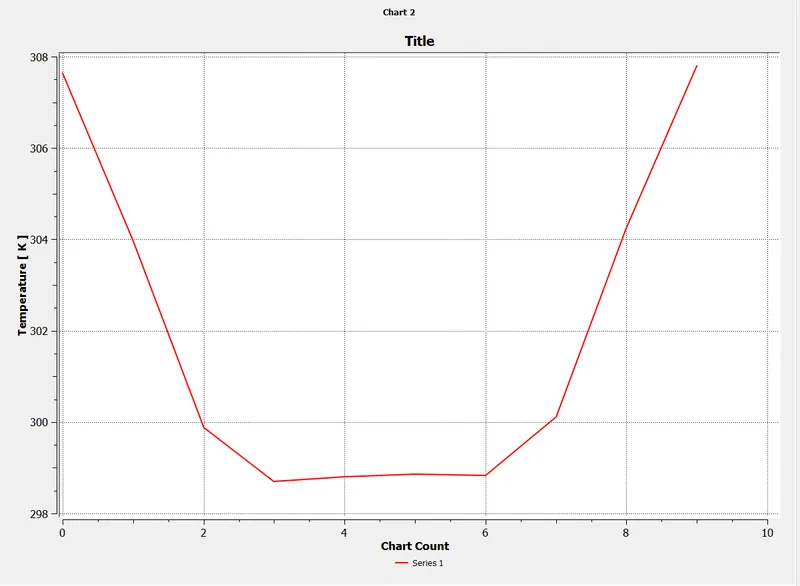
Temperature along the Cross-section of the pipe
Line chart of Temperature along the length of the pipe
Temperature along the Cross-section of the pipe
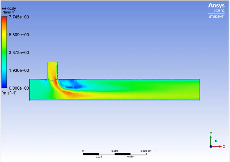
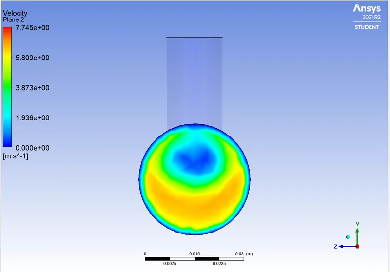
Velocity contour along the length of the pipe
Velocity contour along the cross-section of the pipe
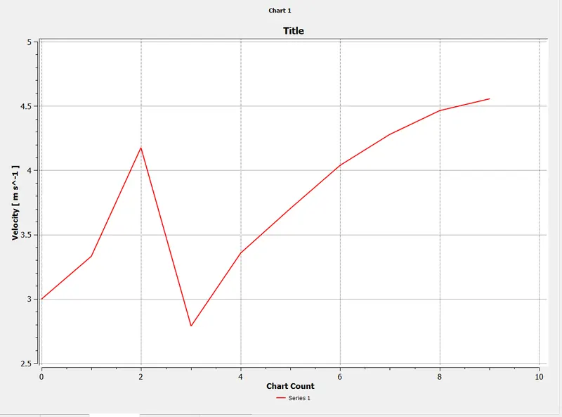
Line chart of velocity along the length of the pipe
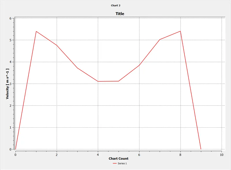
Line chart of velocity along the cross-section of the pipe
************************************CASE 2.2*********************************************
Momentum Ratio = 4
Inlet-x
Velocity = 3m/s
Temperature = 36*C
Inlet-y
Velocity = 12 m/s
Temperature = 19*C
Outlet
Guage pressure = 0
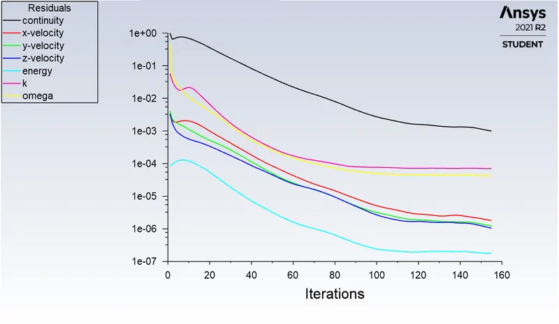
Residuals
Standard Deviation of Temperature
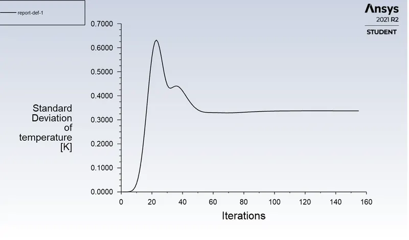
Temperature - 0.6500 K
Area Weighted average of temperature
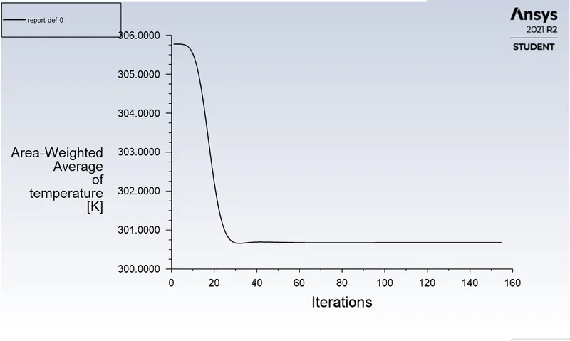
Temperature = 300.05 K
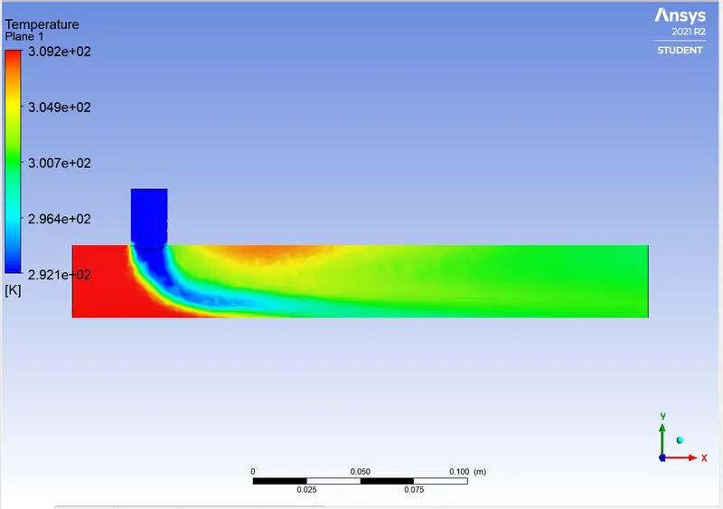
Graphical Representation of Results
Temperature contour along the length of the pipe
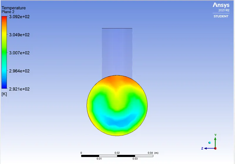
Temperature contour along the cross section of the pipe
Line chart of Temperature along the length of the pipe
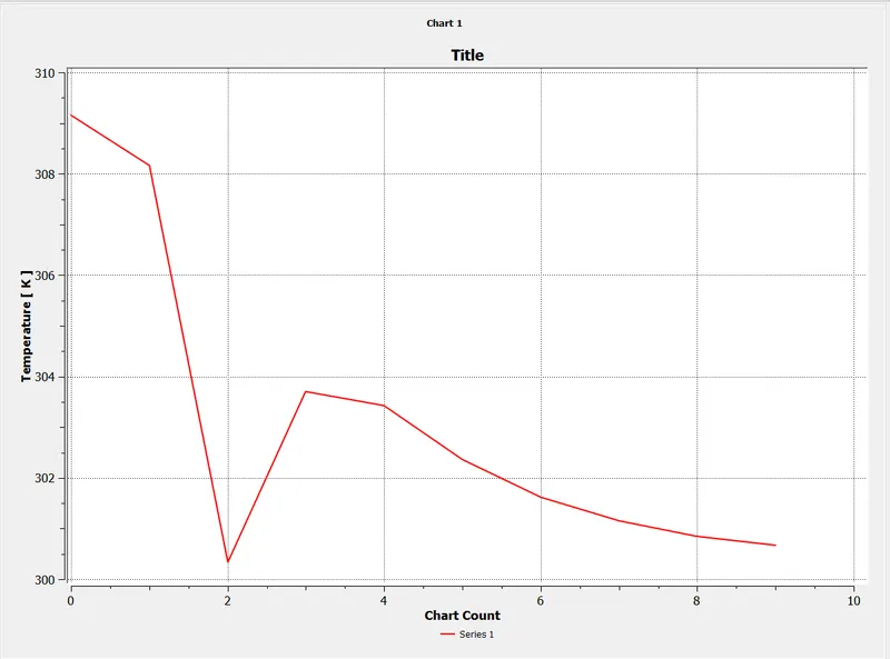
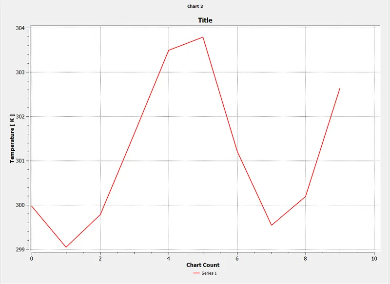
Line chart of temp along the cross section of the pipe
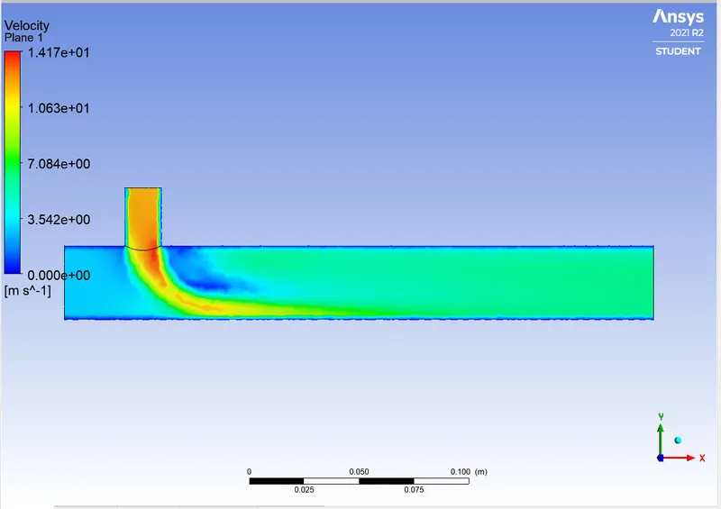
Velocity contour long the length of the pipe
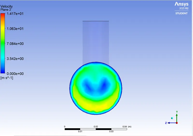
Velocity cross section
Velocity along the length of the pipe
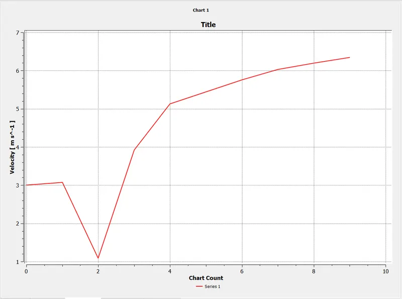
Velocity along the cross section of the pipe
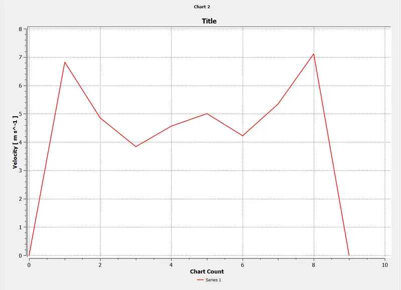
Table comparing K Models on both Long Tee and Short Tee
Short Tee with K omega Model Long Tee with K Omega model
MR = 2 MR = 4 MR = 2 MR = 4
Average Weighted 30.25 27.35 30.45 26.9
Temperature
Cell Count 39375 39375 55759 55759
Number of Iterations 100 225 130 150
to Converge
Standard deviation of 1.800 K 0.9500 K 1.72 K 0.65000 K
temperature
Mesh Independent Study
Long Tee using K omega model
Momentum Ratio = 4
Boundry Conditions
Inlet-x
Velocity = 3m/s
Temperature = 36*C
Inlet-y
Velocity = 12 m/s
Temperature = 19*C
Outlet
Guage pressure = 0
Mesh Size taking = 3mm, 4mm and 7mm
3mm mesh size
Residuals
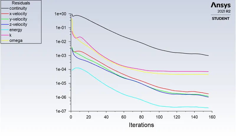
Number of iterations to converge = 150
Standard Deviation of Temperature
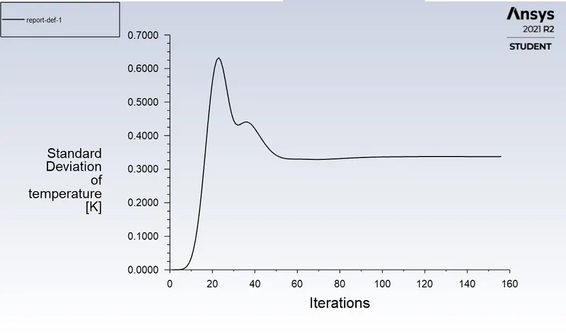
Standard Deviation of Temperature is = 0.3500K
Area-Weighted average of temperature
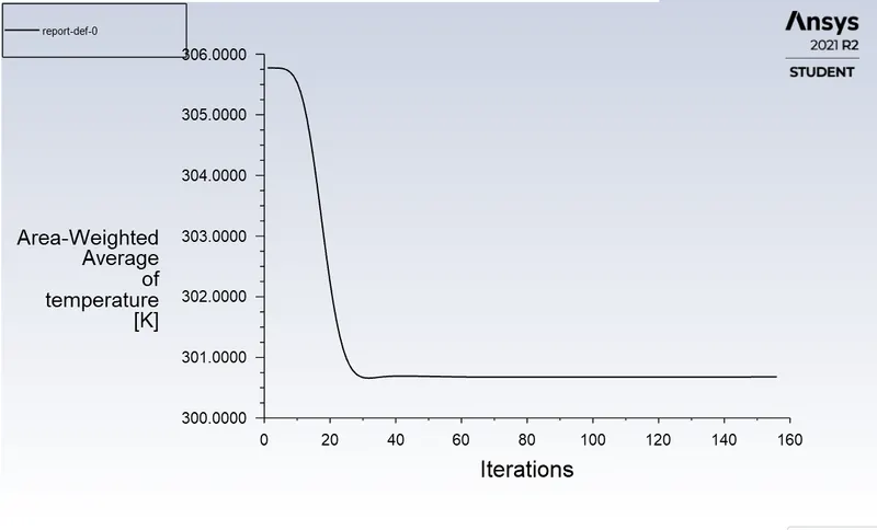
Area- weighted average of temperature = 300.700 K
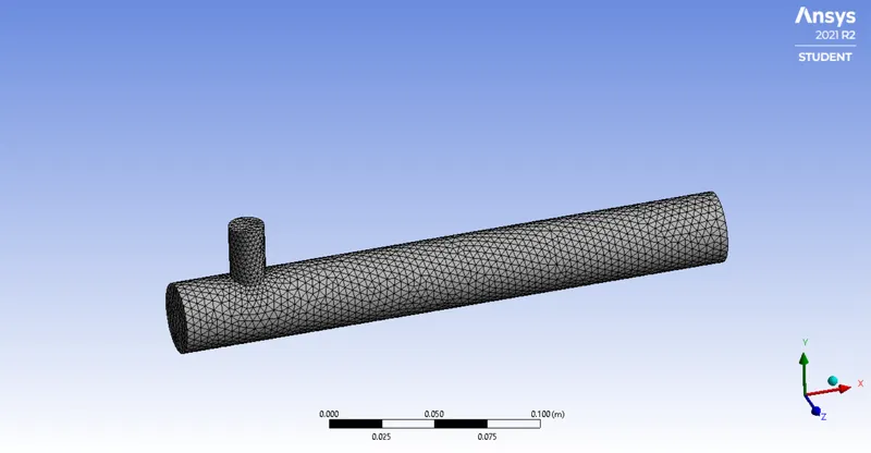
4mm Mesh size
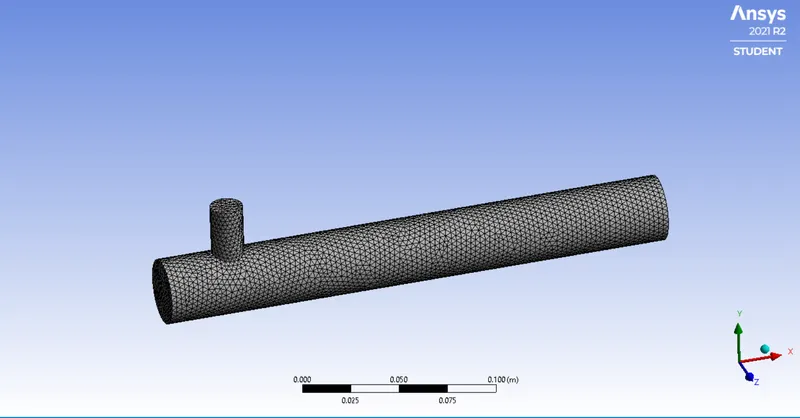
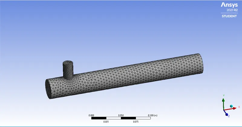
Mesh
Residuals
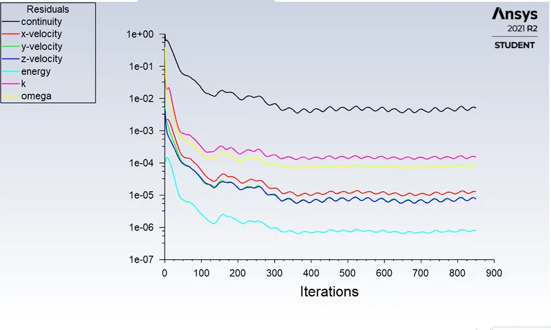
Iterations to converge = 400
Area-Weighted average of temperature
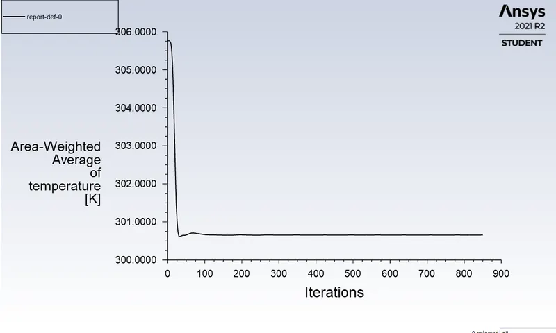
Temperature is = 300.600 K
Standard Deviation of Temperature
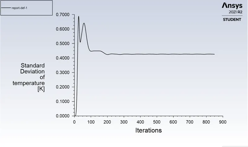
Temperature is = 0.435000 K
7mm Mesh Size
Residuals
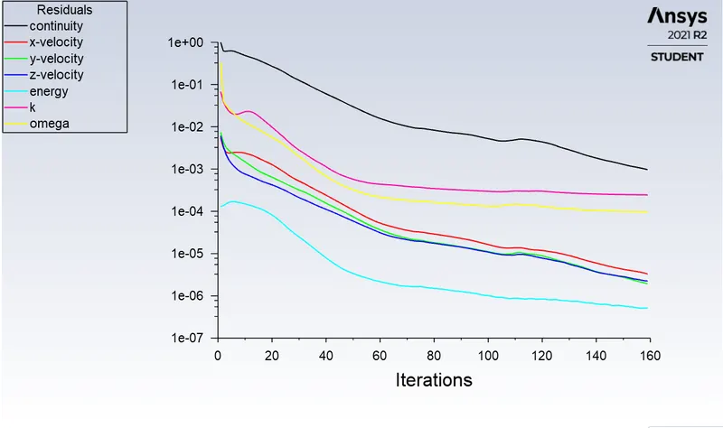
solution did not converged
Standard Deviation of Temperature
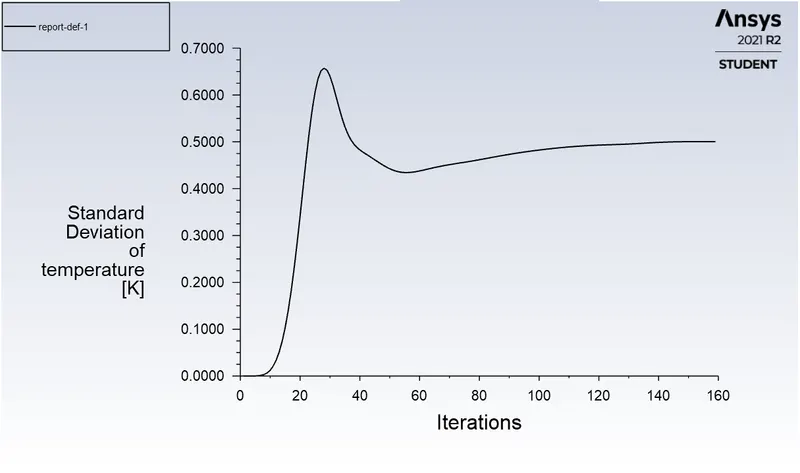
Temperature is = 0.500 K
Area-Weighted average of Temperature
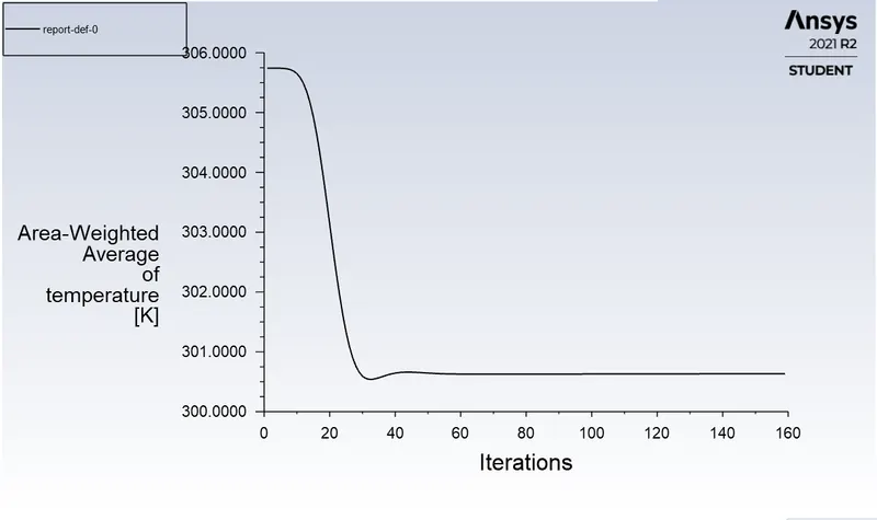
Temperature is = 300.500 K
Comparing results of different mesh sizes
3mm 4mm 7mm
Average weighted 300.700K 300.600K 300.500K
Temperature
Number of cells 55759 28837 15289
Standard Deviation 0.3500K 0.435000K 0.500K
of Temperature
On Changing the mesh size and making the mesh finer, we can see that, by changing size from 4mm to 3mm, the average weighted temperature remains almost same. Thus we can conclude that the grid dependency is achieved further refinement of mesh will not affect the results much, it will just increase the number of elements and computational time.
Conclusion
On reviewing all the above cases, it is confirmed that the increase in length resulted in better mixing of fluid although there is not much difference in average outlet temperature with a specific momentum ratio.
The standard deviation of the longer tee is lesser than the shorter tee in all the conditions. There are more orange zones in a shorter tee than in a longer tee. But with the higher momentum ratio not only the mixing of fluids happened efficiently but even there is a significant drop in the average outlet temperature. Longer Tee with a higher momentum ratio produced a better result than the rest other cases.