Challenge

Week 1- Mixing Tee

PP J Phani Virat30 Sept 2021

MIXING TEE EFFICIENCY

To set up steady-state simulations to compare the mixing effectiveness in a Tee shape mixing CAD model when hot inlet temperature is 36⁰C & the Cold inlet is at 19⁰C. Using the k-epsilon and k-omega SST model for the first case and based on your judgment use the more suitable model for further cases. Giving the reason for choosing a suitable model is compulsory.

GIVEN DATA:

Hot air inlet temperature = 36°c
Cold air inlet temperature = 19°c
Hot air inlet velocity = 3 m/s
Momentum Ratio = 2 and 4 (Ratio of V(input) max and V(input)min

CAD MODEL AND GEOMETRY:

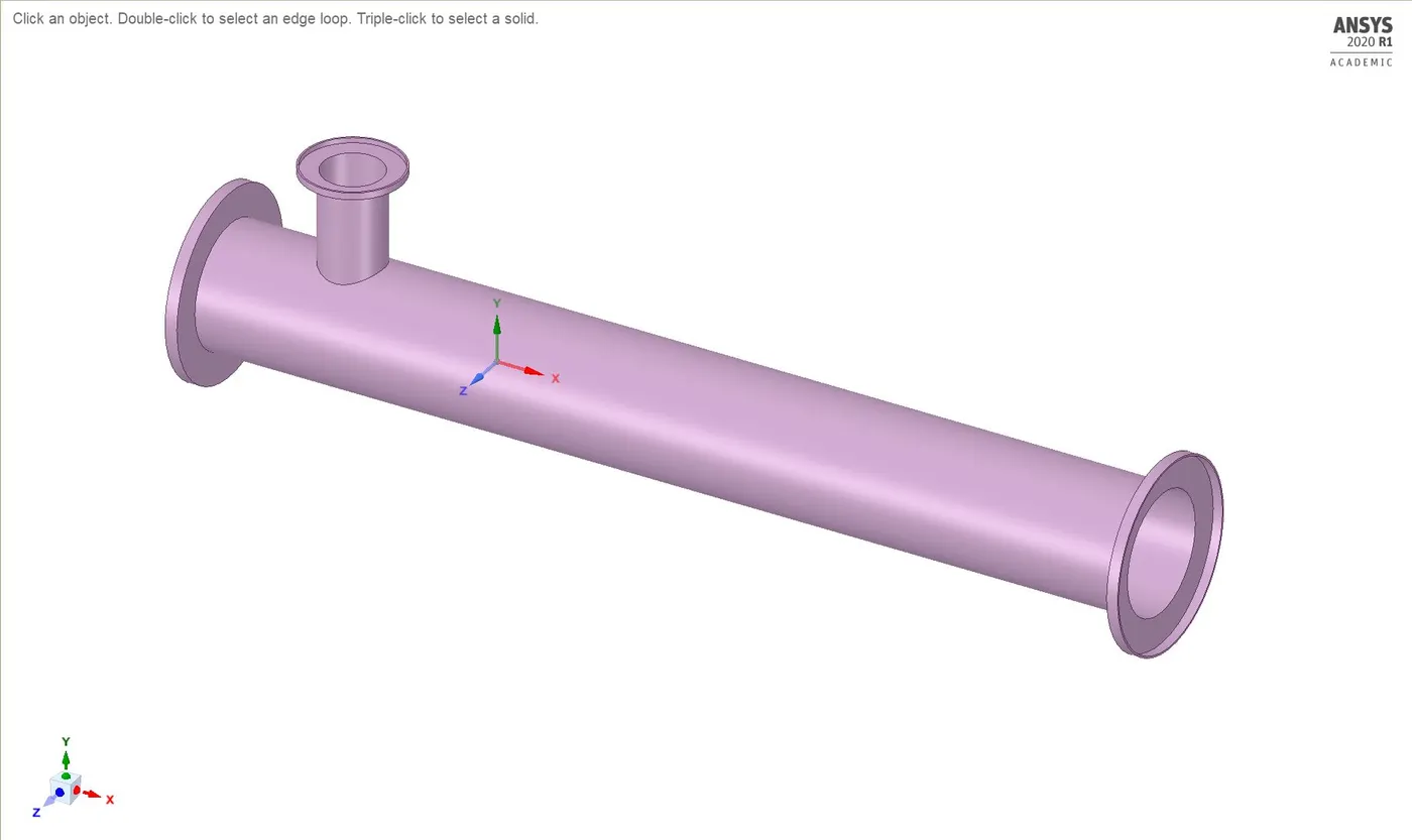
CAD solid model of the actual Tee shaped pipe with two inlets and outlet for mixing of two streams at different temperatures

VOLUME EXTRACTION:

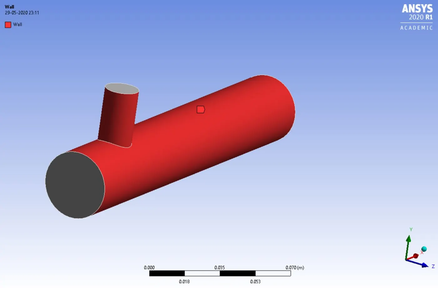
The CFD of the hollow region is the actual region in which the hot and cold fluid flow analysis can be done. Thus the solid model shown below is the actual volumetric region through which the fluid flows and which actually needs to be meshed and analysed for its temperature and velocity profiles at various regions.

MESHING DETAILS:

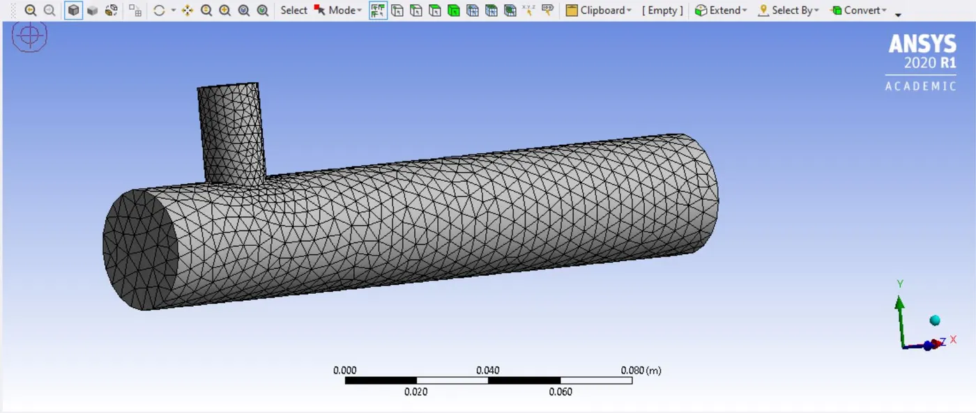
3D meshing of the volume extracted material in ANSYS mesh

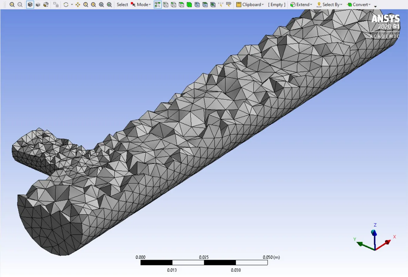
The sectional trapezoidal elemental face version of the meshing showing the better view of the 3D volumetric meshing of the cad model

The meshing done after the naming of the different parameters shows the specifications of the volumetric mesh done by showing the number of nodes, elements and faces of the whole meshed component and its meshing quality which further decides the better resolution and preciseness of the solution calculations, the convergence of the residuals and the post analysis as well at last. Thus the very preciseness and more detailed result is much dependent on the meshing quality of the CAD model.

GEOMETRY	SHORTER LENGTH MODEL	LONGER LENGTH MODEL
NUMBER OF NODES	3142	3495
NUMBER OF ELEMNTS	14247	15689
ELEMENT SIZE	5 mm	13.853

Table: Table for the comparison of the two different design meshing values and details.

The meshing details shown above in the table shows that even though the element size of the bigger CAD model is more than 2.5 times of the smaller model still the smaller model have comparable or almost same number of nodes and elements. This clearly depicts that when size of an element is reduced or increased how it drastically effects the number of elements and the nodes

MESHING QUALITY:

The below histogram shows he quality of mesh by comparing the elements metrics to the number of elements which shows the minimum % of elements with 28% element with the smallest number of element sizes with poor quality. This lowest % should be generally above 50% for the good meshing or around 40%.

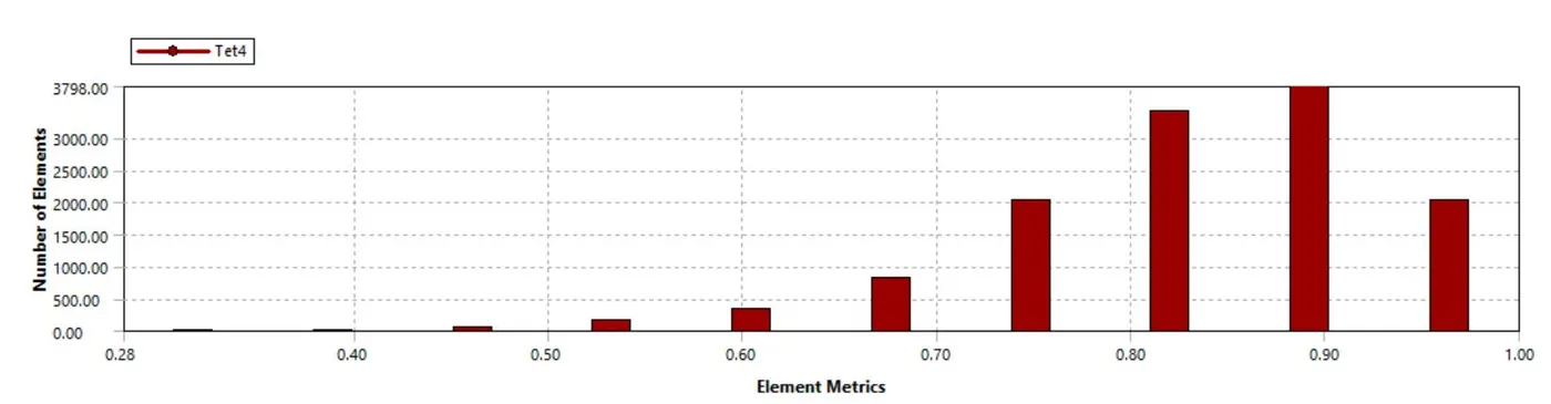
Meshing quality of the shorter model

The min value for the element metrics for the short Tee is .28 and the max is 1as seen from the mesh quality histogram.

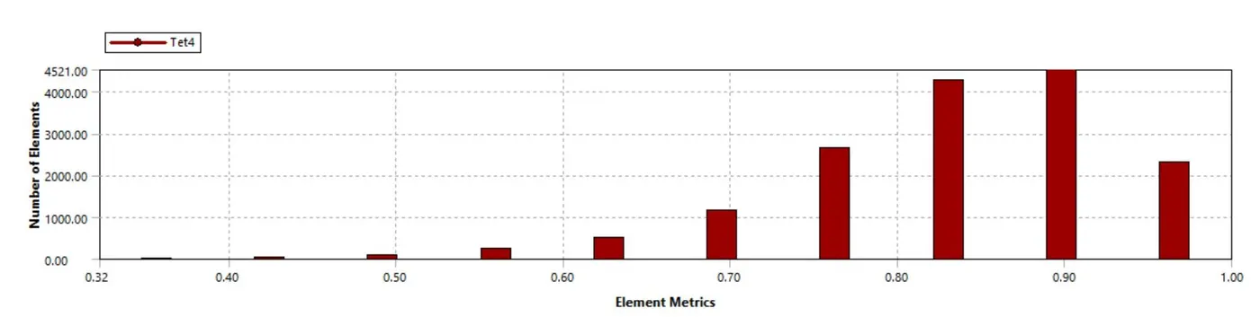
Meshing quality of the longer CAD model

The min value for the element metrics for the long Tee is .32 and the max is 1 as seen from the mesh quality histogram.

SETUP:

Steady state pressure based absolute velocity formulation type solver is being used for both type of models so as per the same given conditions the comparison of the analysis can be further carried out. Energy has been included and considered for the solution part and a residual plot has been also plotted for various cases further.

PHYSICS :

The comparative studies of two designs have been studied by the use of k-omega and k-epsilon model-epsilon model here used is the realizable with standard wall function for near wall treatment and SST k-omega model. Here Shear Stress Transport (SST) is a variant of standard k-omega model. SST is recommended generally for high accuracy boundary layer simulation.

MATERIAL:

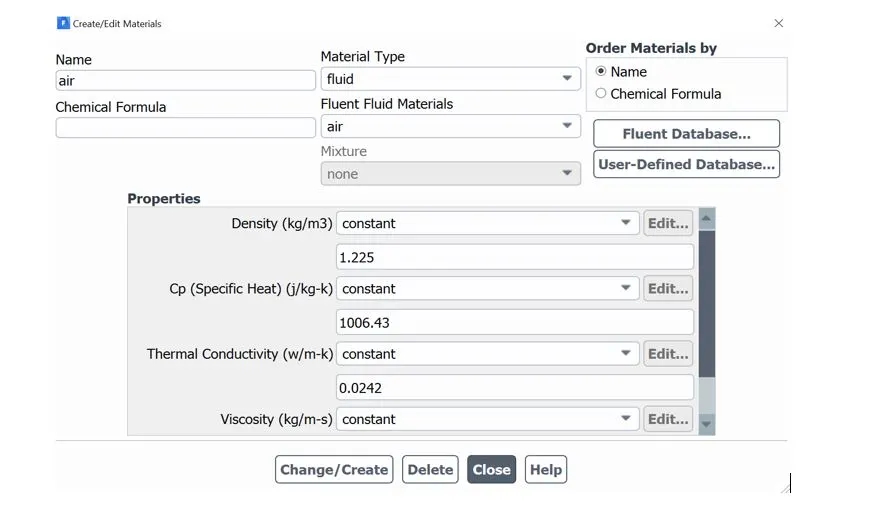
Fig: Material used as a fluid for simulation

BOUNDARY CONDITIONS:

The given below boundary conditions are being used for calculation and simulation for both designs and the specific models as well.

BOUNDARIES	VELOCITY	TEMPERATURE
INLET-X	3 m/s	36°C
INLET-Y	6m/s & 12m/s	19°C

Table: Boundary conditions table

RESULTS AND DISCUSSIONS (SHORT & LONG TEE MODEL) FOR TOTAL 5 CASES

CASE 1: SHORT TEE GEOMETRY WITH MOMENTUM RATIO =2 USING K-epsilon MODEL

In this case shorter length Tee geometry was considered with a momentum ratio of 2 whereas temperature of inlet hot air was 36 °C with an incoming velocity of 3m/s. The temperature of cold inlet air was 19°C with an incoming velocity of 6m/s. the residual variables values are being shown on the plot below which shows how the residuals gets converged after certain iterations to give the stable value of temperature at outlet with the minimum standard deviation possible for comparative models.

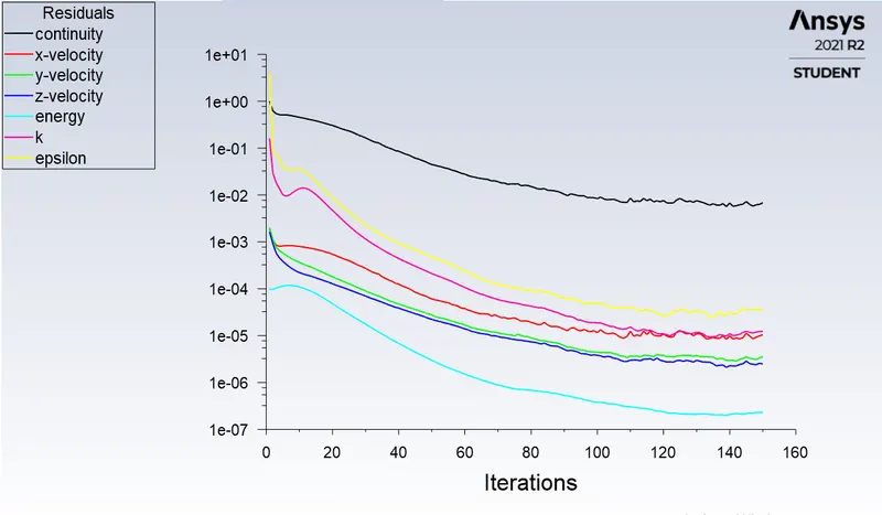
Fig: Residual plot in case of short Tee for momentum ratio: 2 for K-epsilon Realizable Model.

As seen from the above plot we can say that the convergence started somewhere around the iterations of 120 and after that there is very negligible changes in the residual values w.r.t to the further iteration

The below fig shows the Area-weighted average for the temp outlet is around 30.2539°C and standard deviation is around 1.211075°C.

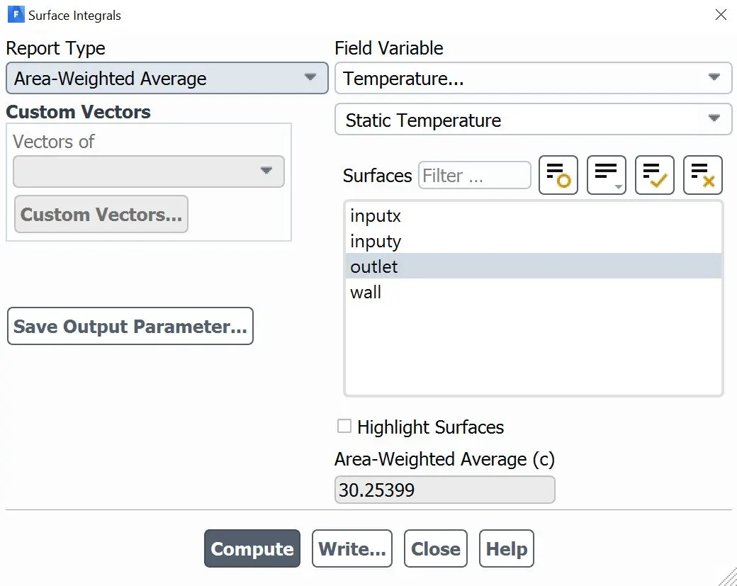
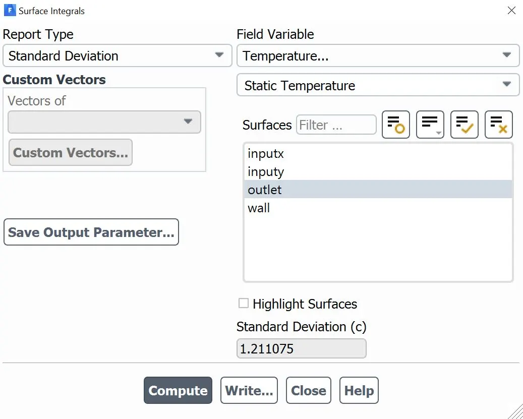
Fig: the area weighted average value of temperature and its standard deviation for the OUTLET

PLOTS:

The below plots shows the area weighted average of the temperature at the outlet zone. This value basically shows the change in temperature w.r.t to the iterations which after converging after a certain point shows the outlet temperature goes stable now onwards after around 100 iterations as per the plot below

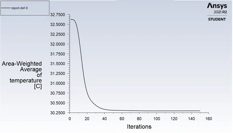
Fig: The area-weighted average for temperature at outlet.

The below plots shows the standard deviation of the temperature at the outlet zone. This value basically shows the change in deviation of temperature w.r.t to the iterations which after converging after a certain point shows the outlet standard deviation of temperature goes stable now onwards after around 500 iterations as per the plot below.

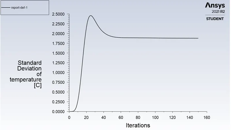
Fig: Standard deviation of temperature at outlet with the number of iterations

The following plots shows the variation of temperature and velocity on a plane generated between the geometry. This is the plane that divides the geometry into two equal halves. The variation of temperature (user specified) and velocity (global) has been plotted.

Why global? The reason why the velocity isn’t user specified btw 3m/s -6m/s is that we also do need to know the stagnation points for the whole flow model here. The points where the velocity is almost zero or where there is no-slip condition.

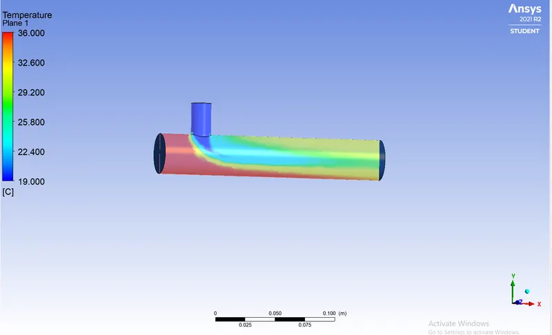
Fig: Temperature variation from 19 deg C to 36 deg C in the plane region

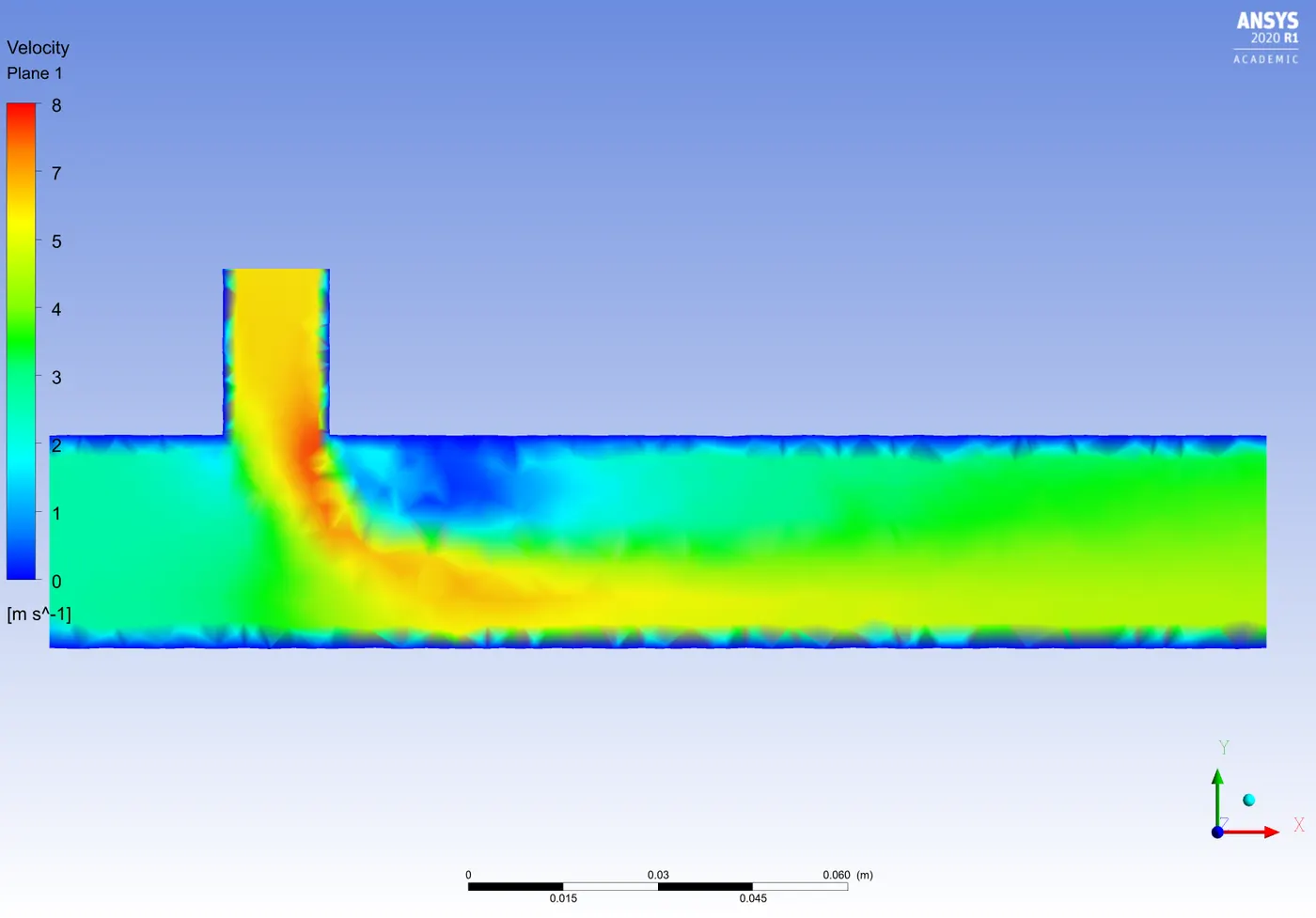
Fig: Velocity variation in global reference in the plane region.

The region attracted to the wall or on the wall shows the region of almost no-slip condition and have almost zero velocity and comparatively very lesser temperature distribution or mixing takes place in this region. These regions can also be referred to as the stagnation points. This is why to study the nature of simulation the legend limits for the velocity profile has been set global and not user specified. If the limits for velocity would be set to user specified then that would not give us the exact region of the zero velocity profile area and thus no significant stagnation points would be clearly be achieved.

contour plot & line plots

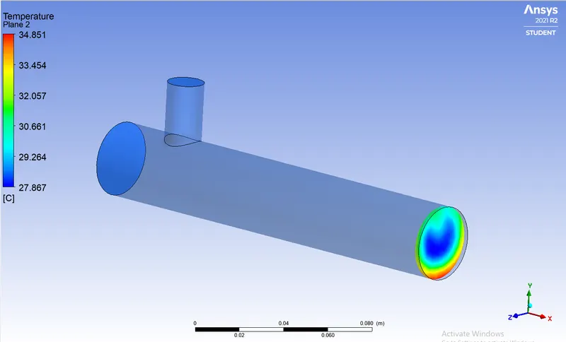
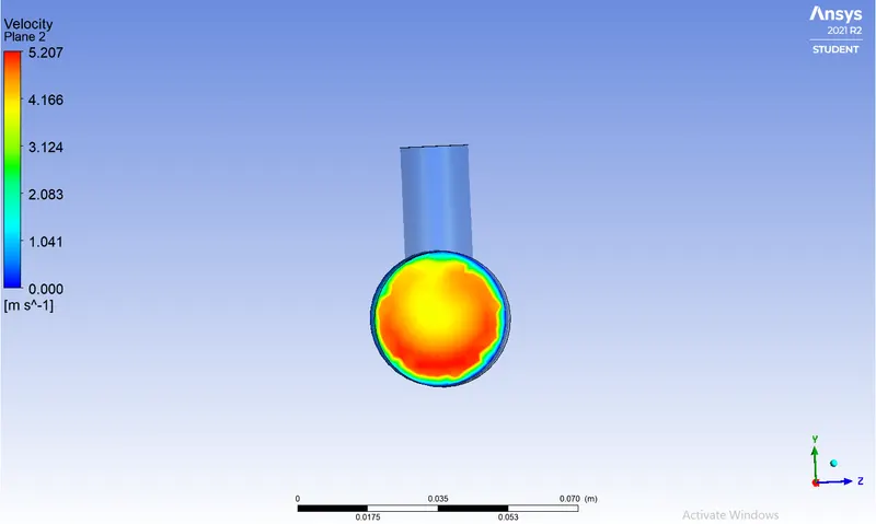
Temperature contour plot Velocity contour plot

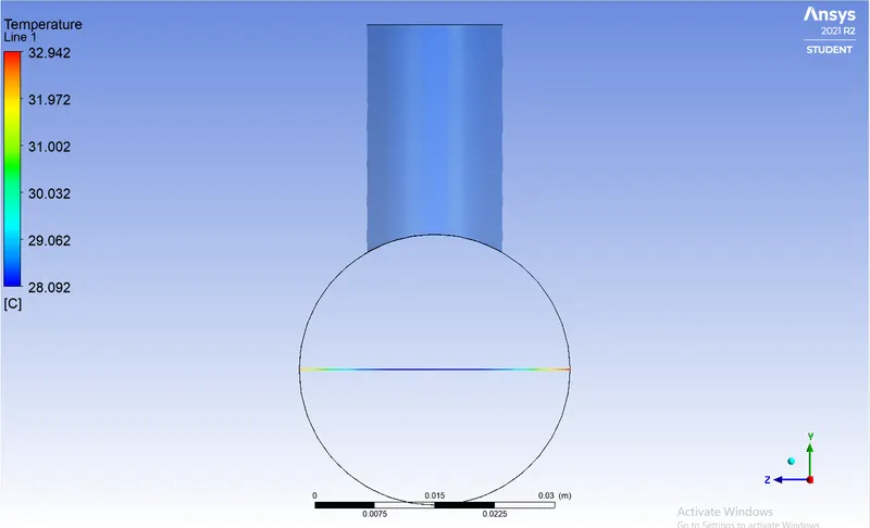
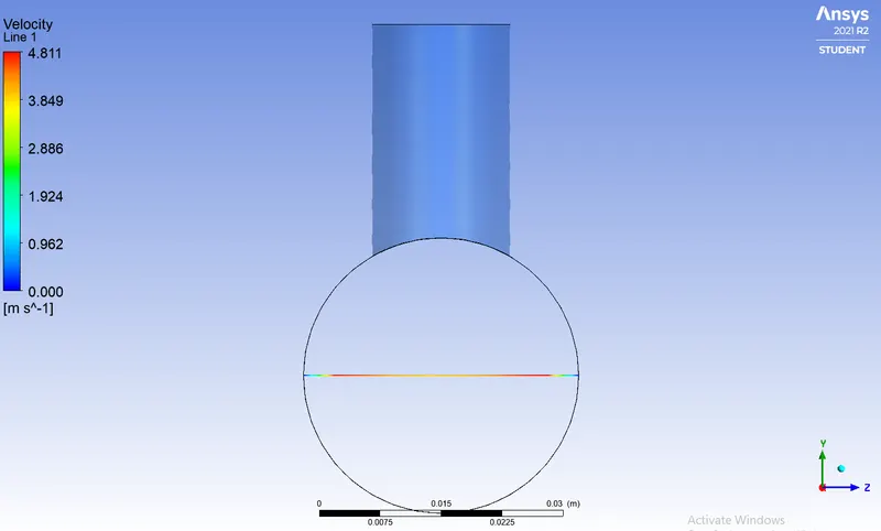
Temperature line plot across the pipe Velocity line plot across the pipe

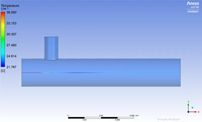
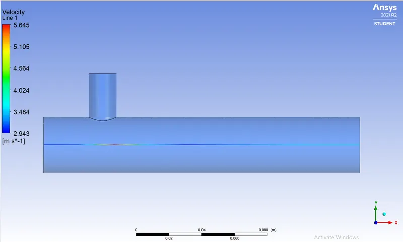
Temparature line plot along the pipe Velocity line plot along the pipe

CASE 2: SHORT TEE GEOMETRY WITH MOMENTUM RATIO =2 USING K-omega MODEL

In this case shorter length of geometry was considered with a momentum ratio of 2. The temperature of inlet hot air was 36 degree-centigrade with an incoming velocity of 3m/s. The temperature of cold air was 19 deg C with an incoming velocity of 6m/s. Fig. below shows the residual plot. The simulation was run for more than 150 time-step in order to confirm for convergence of simulation results. The simulation was converged after running it for 120 iteration. It can be observed from residual plot, all parameters are converging its value after 120 iterations and further.

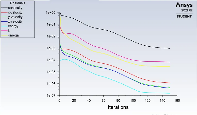
Fig: Residual plot in case of short Tee for momentum ratio: 2 for K-omega, SST Model

PLOTS:

This model shows that it took much more number of iterations in this case to converge to the solution for the residuals as compared to the previous method. Area weighted temperature for output is 30.25°C

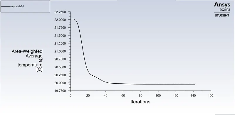
Fig: Area weighted average for temperature for the outlet.

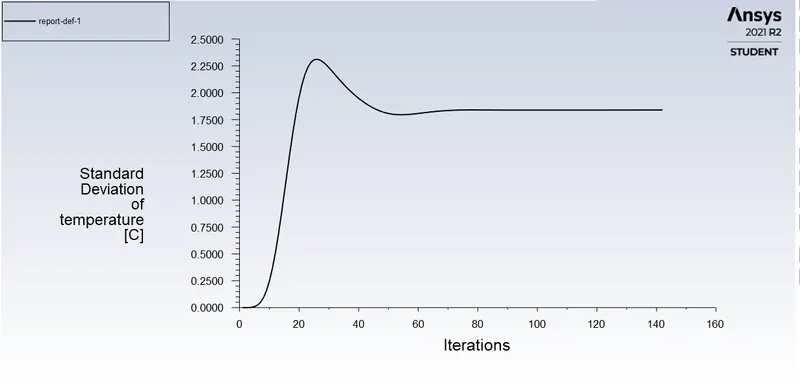
Fig: Standard deviation of temperature at outlet with the number of iterations

Thus as seen from the area-weighted plot and standard deviation plot we can say that the deviation in the temperature for output is very large as compared to the previous model that was k-epsilon model.

Thus as per the plot and the time consumption the k-epsilon model seems to be more effective here for the momentum ratio of 2. Also the standard deviation for the model is around 2.01°C for the temperature at the outlet.

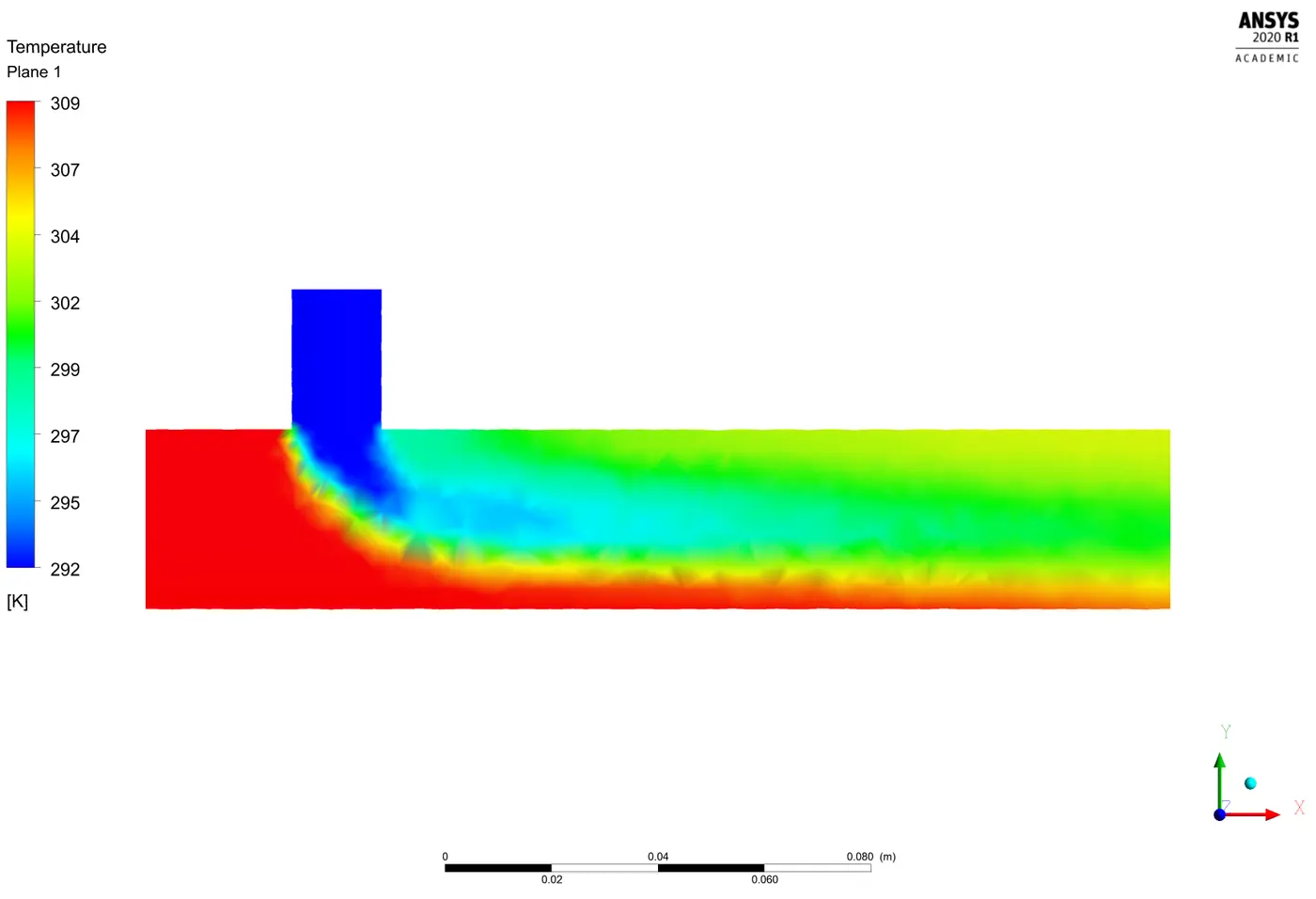
Fig: Temperature variation from 19 deg C to 36 deg C in the plane region

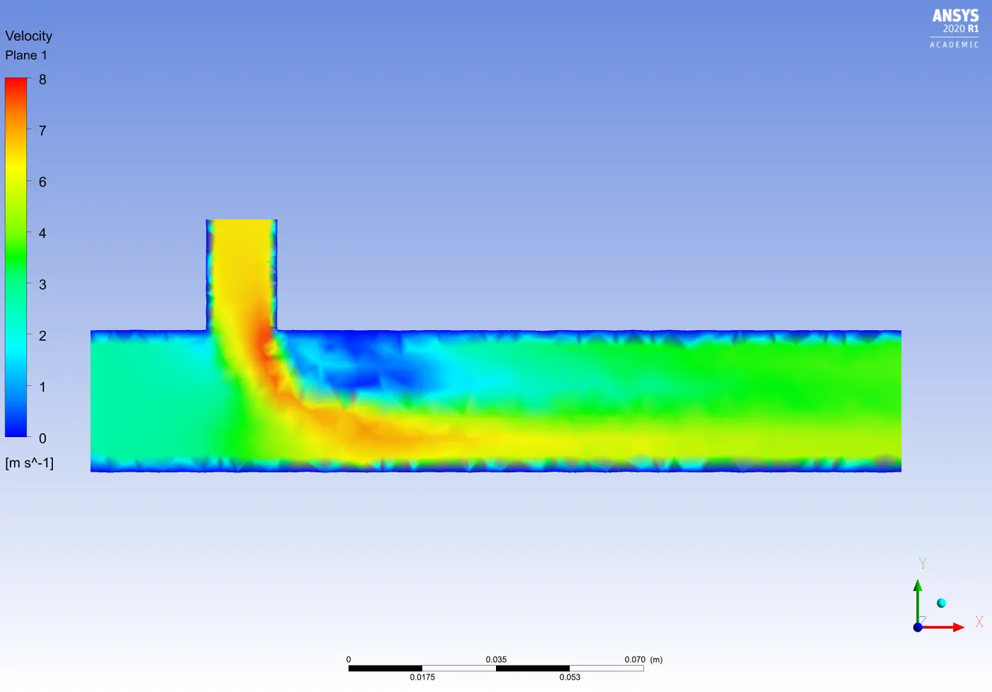
Fig: Velocity variation in global reference in the plane region.

contour plot & line plots

Temperature contour plot Velocity contour plot

Temperature line plot across the pipe Velocity line plot across the pipe

Temparature line plot along the pipe Velocity line plot along the pipe

With that we can conclude K-epsilon model will converge more faster than the K-Omega model and for wall funtions we use K-omega model and away from the wall we use k-epsilon and here we are calculating the Temparature so we can use the k-epsilon model

CASE 3: SHORT TEE GEOMETRY FOR MOMENTUM RATIO =4, USING K-epsilon MODEL

In this case shorter length of geometry was considered with a momentum ratio of 4. The temperature of inlet hot air was 36 degree-centigrade with an incoming velocity of 3m/s. The temperature of cold air was 19 deg C with an incoming velocity of 12 m/s. Fig. below shows the residual plot. The simulation was run for more than 500 time-step in order to confirm for convergence of simulation results. The simulation was converged after running it for 150 iteration. It can be observed from residual plot, all parameters are converging its value from 120 to further iterations.

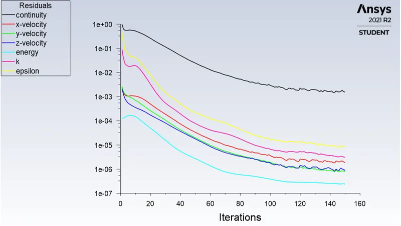
Fig: Residual plot in case of short Tee for momentum ratio: 4 for K-epsilon Realizable Model.

PLOTS:

This model shows that it took much lesser number of iterations in this case to converge to the solution for the residuals as compared to the previous boundary conditions. Area weighted temperature for output is 27.54°C and standard deviation is 1.37455°C.

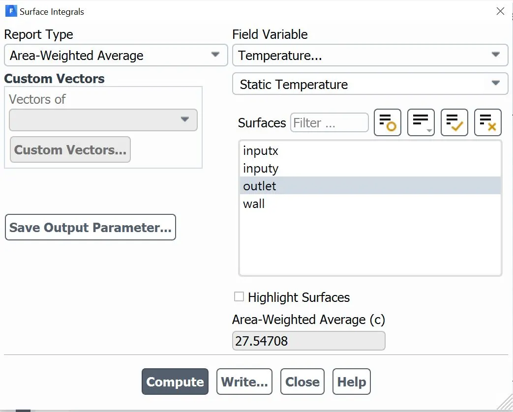
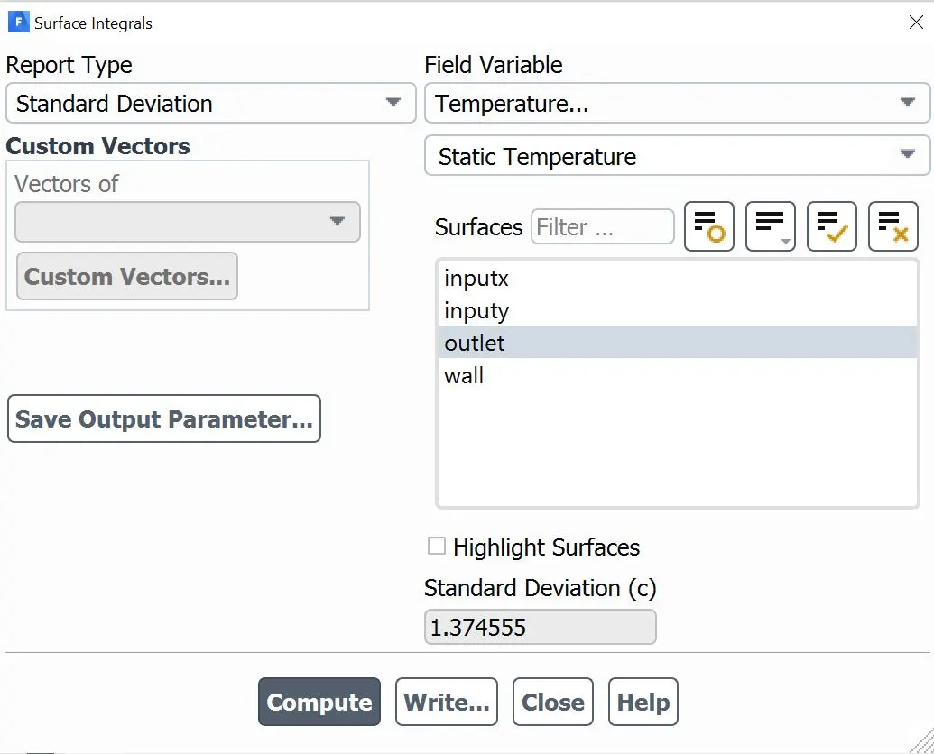
Fig: Area weighted average for output temperature and its standard deviation

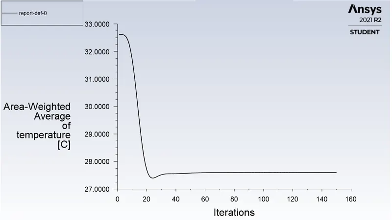
Fig: The area-weighted average for temperature at outlet

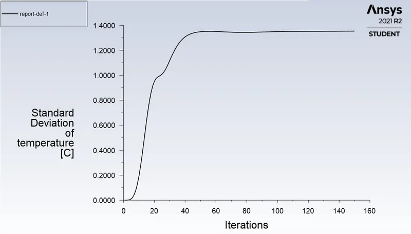
Fig: Standard deviation of temperature at outlet with the number of iterations

The following plots shows the variation of temperature and velocity on a plane generated between the geometry. The variation of temperature (user specified) and velocity (global) has been plotted.

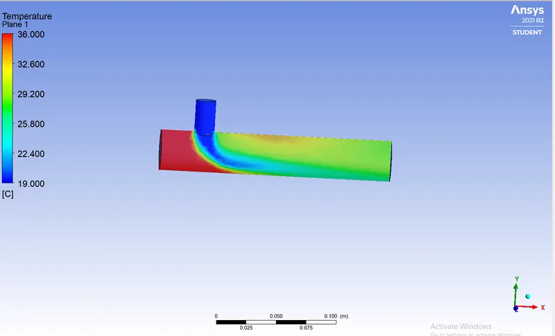
Fig: Temperature variation from 19 deg C to 36 deg C in the plane region

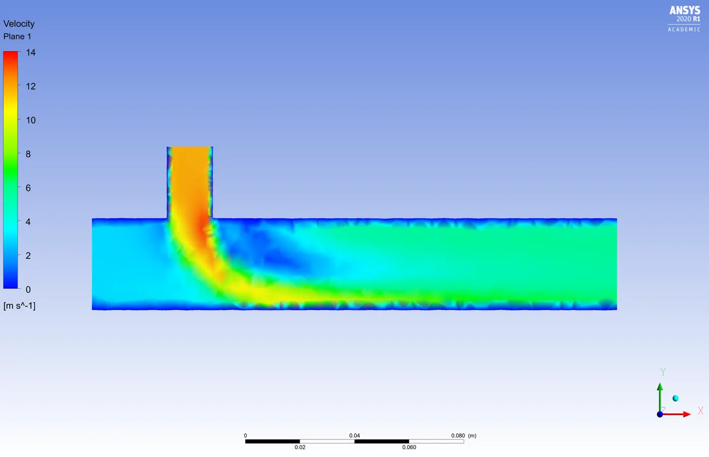
Fig: Velocity variation in global reference in the plane region.

contour plot & line plots

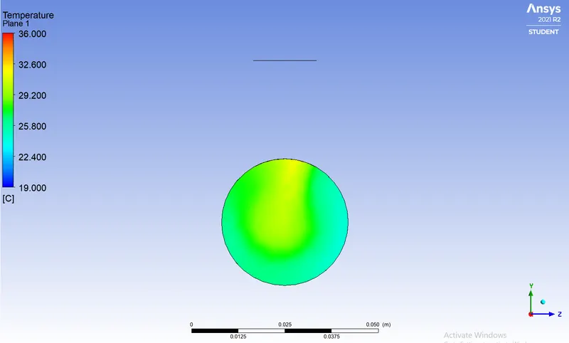
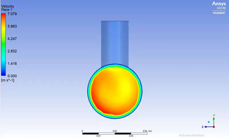
Temperature contour plot Velocity contour plot

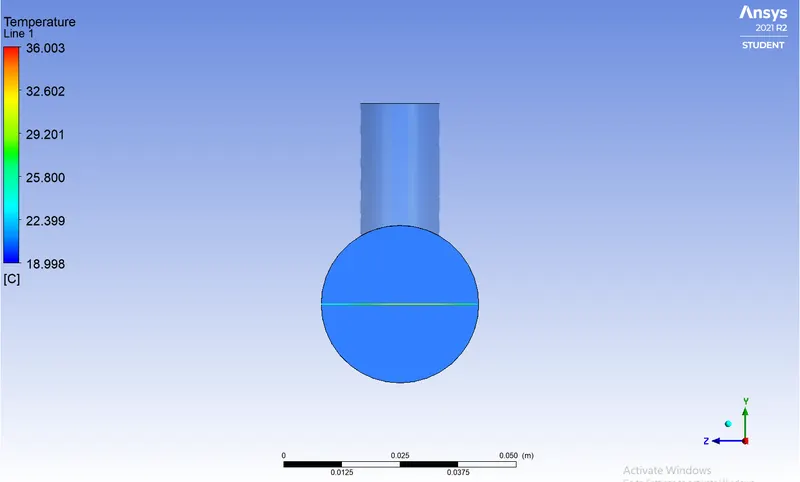
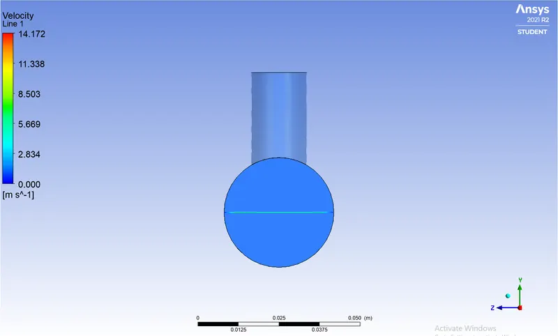
Temperature line plot across the pipe Velocity line plot across the pipe

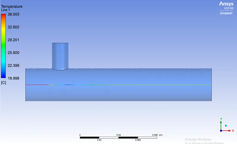
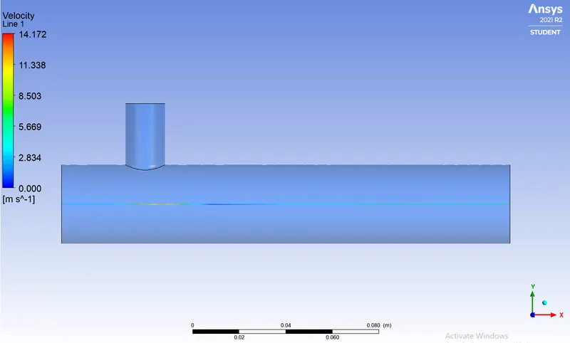
Temparature line plot along the pipe Velocity line plot along the pipe

CASE 4: LONG TEE GEOMETRY WITH MOMENTUM RATIO =2, USING K-epsilon MODEL:

In this case longer length of geometry was considered with a momentum ratio of 2. The temperature of inlet hot air was 36 degree-centigrade with an incoming velocity of 3m/s. The temperature of cold air was 19 deg C with an incoming velocity of 6 m/s. Fig. below shows the residual plot. The simulation was run for more than 140 time-step in order to confirm for convergence of simulation results. The simulation was converged after running it for 120+ iteration. It can be observed from residual plot, all parameters are converging its value after 120 iterations and further.

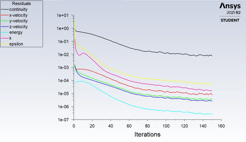
Fig: Residual plot in case of short Tee for momentum ratio: 2 for K-epsilon Realizable Model.

PLOT:

Area weighted temperature for output is 30.2648 °C and standard deviation is 1.354 °C.

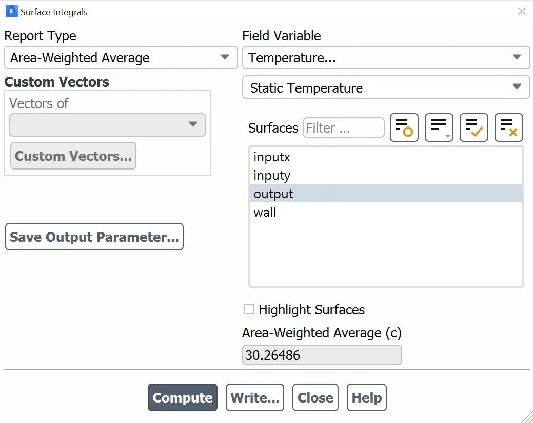
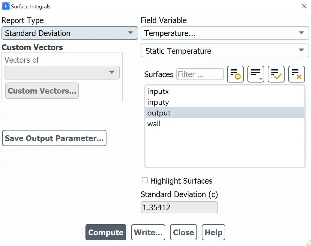
Fig: Area weighted average value of temperature and its standard deviation for the OUTLET

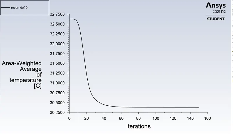
Fig: The area-weighted average for temperature at outlet.

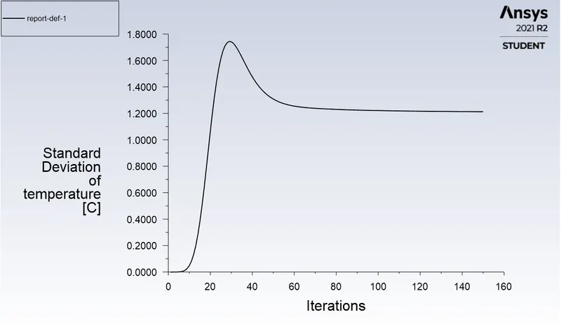
Fig: Standard deviation of temperature at outlet with the number of iterations.

The following plots shows the variation of temperature and velocity on a plane generated between the geometry. The variation of temperature (user specified) and velocity (global) has been plotted.

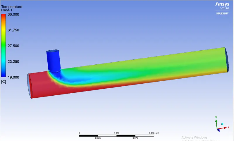
Fig: Temperature variation from 19 deg C to 36 deg C in the plane region.

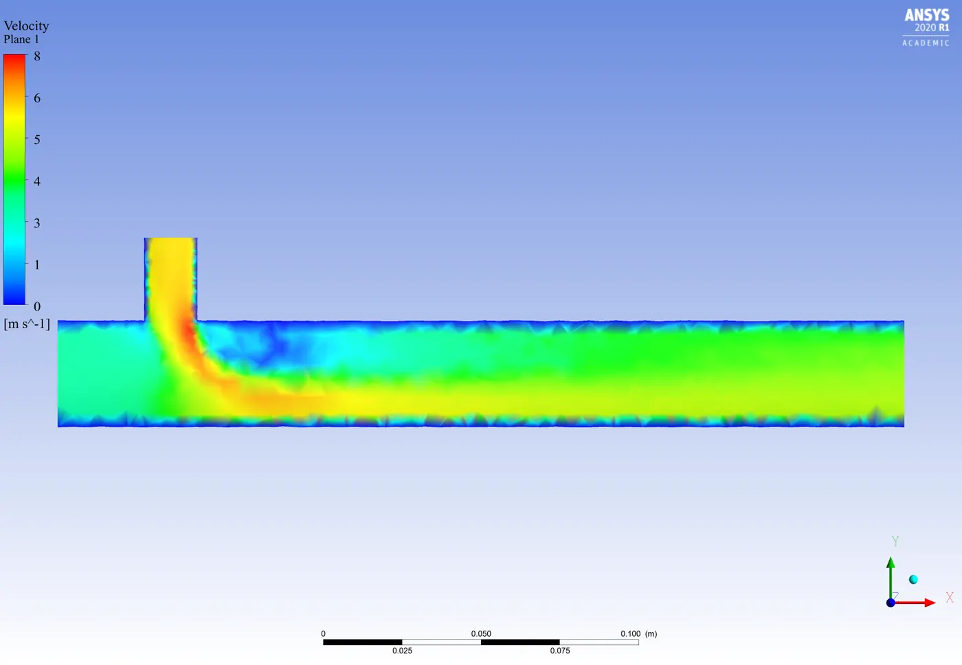
Fig: Velocity variation in global reference in the plane region.

contour plot & line plots

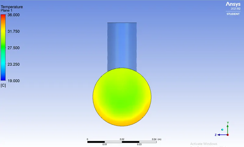
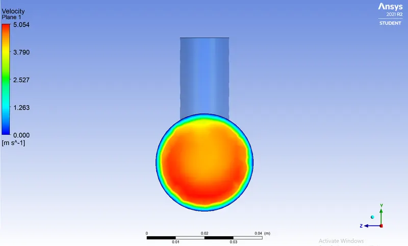
Temperature contour plot Velocity contour plot

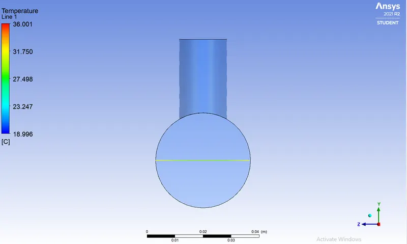
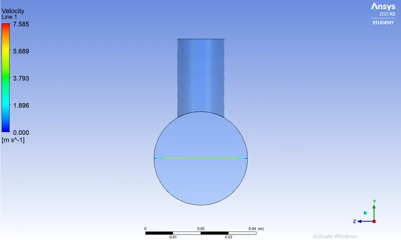
Temperature line plot across the pipe Velocity line plot across the pipe

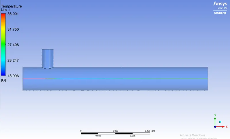
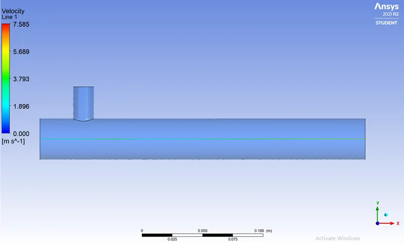
Temparature line plot along the pipe Velocity line plot along the pipe

CASE 5: LONG TEE GEOMETRY FOR MOMENTUM RATIO =4, USING K-epsilon MODEL

In this case longer length of geometry was considered with a momentum ratio of 4. The temperature of inlet hot air was 36 degree-centigrade with an incoming velocity of 3m/s. The temperature of cold air was 19 deg C with an incoming velocity of 12 m/s. Fig. below shows the residual plot. The simulation was run for more than 100 time-step in order to confirm for convergence of simulation results. The simulation was converged after running it for 120+ iteration. It can be observed from residual plot, all parameters are converging its value after 120 iterations and further.

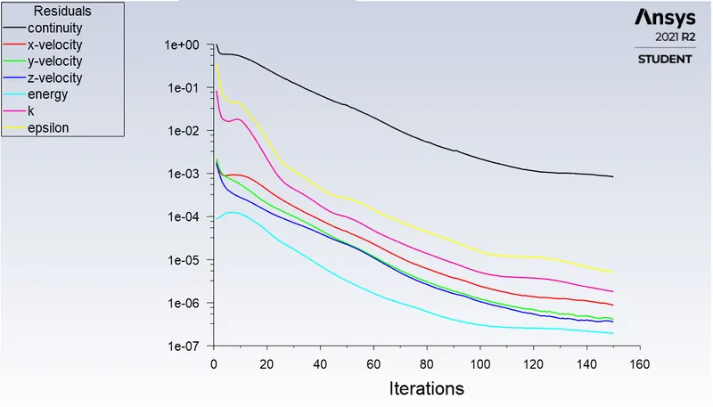
Fig: Residual plot in case of short Tee for momentum ratio: 4 for K-epsilon Realizable Model.

PLOTS:

Area weighted temperature for output is 27.48819 °C and standard deviation is 0.5737452 °C.

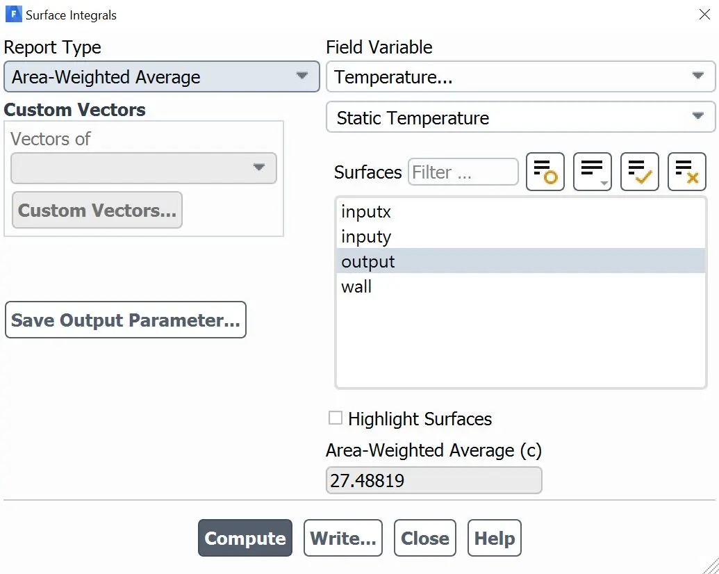
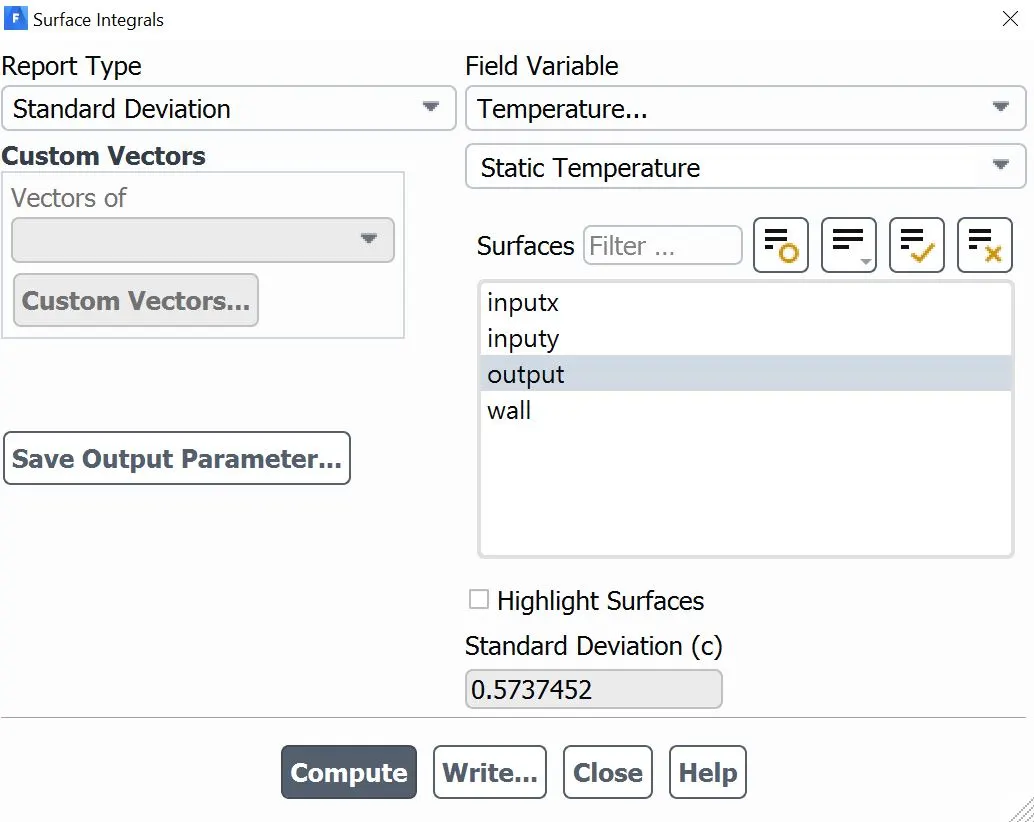
Fig: Area weighted average value of temperature and its standard deviation for the OUTLET.

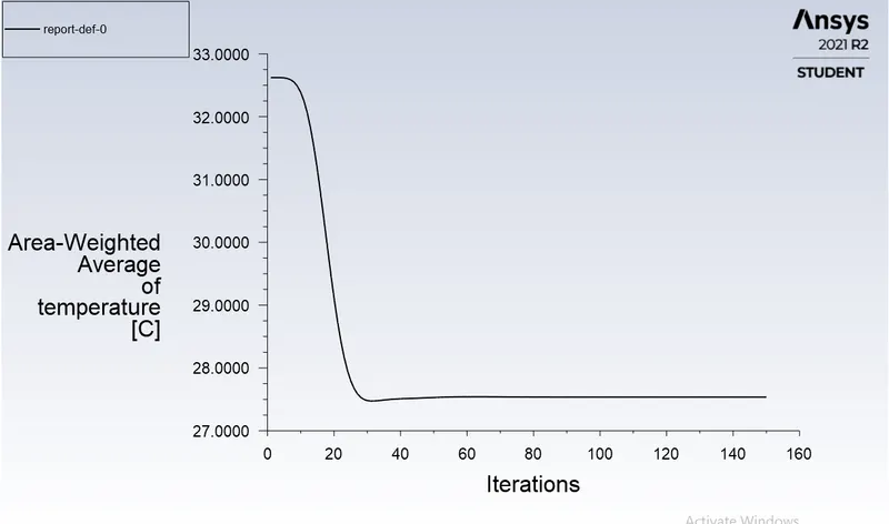
Fig: The area-weighted average for temperature at outlet.

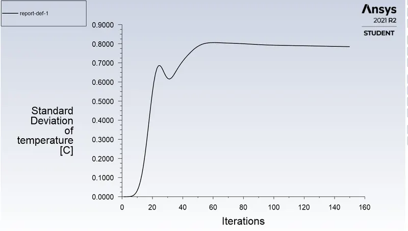
Fig: Standard deviation of temperature at outlet with the number of iterations.

The following plots shows the variation of temperature and velocity on a plane generated between the geometry. The variation of temperature (user specified) and velocity (global) has been plotted.

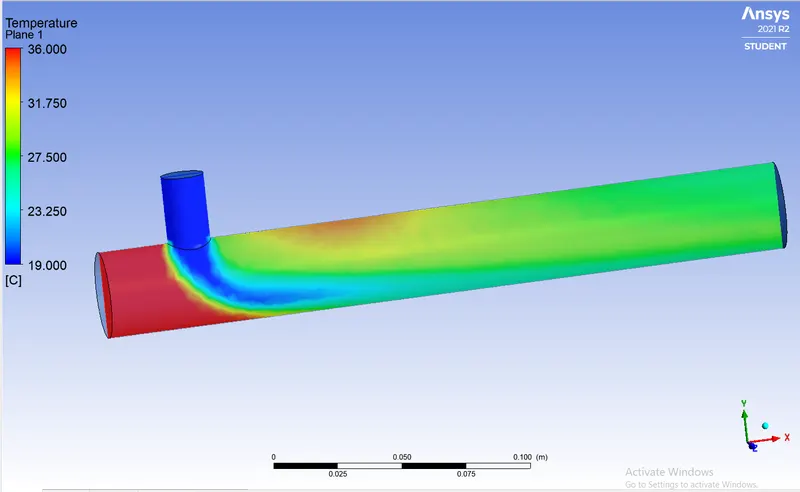
Fig: Temperature variation from 19 deg C to 36 deg C in the plane region.

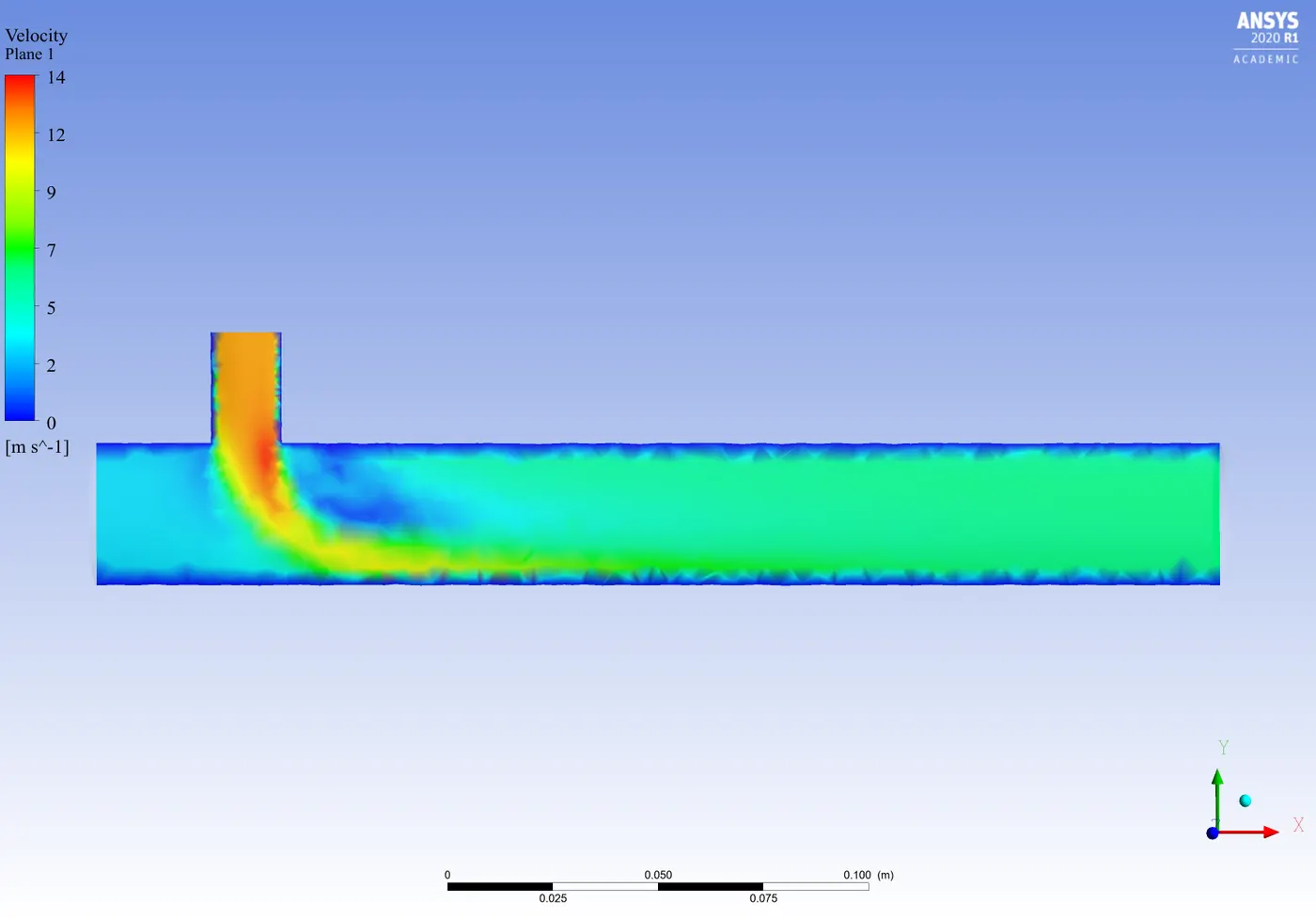
Fig: Velocity variation in global reference in the plane region.

contour plot & line plots

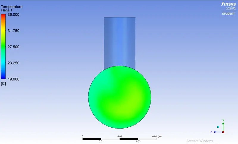
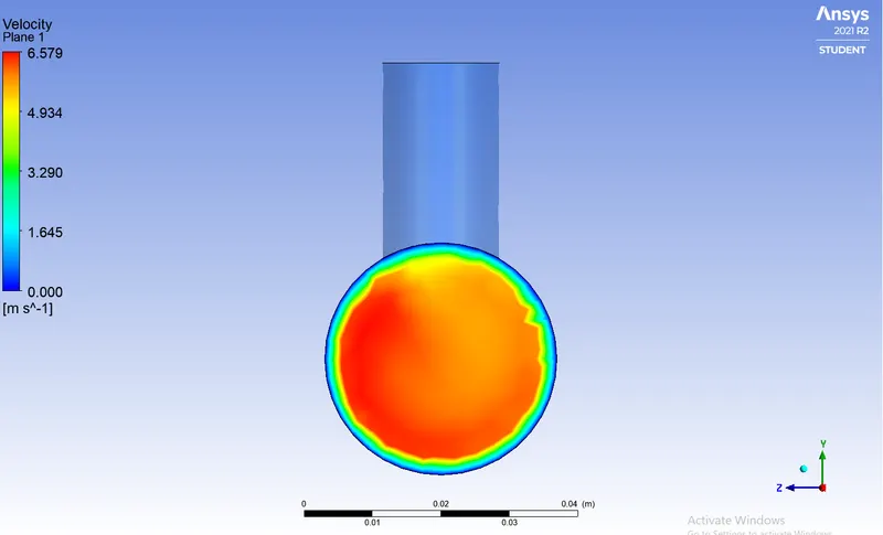
Temperature contour plot Velocity contour plot

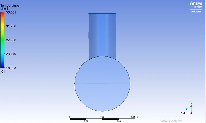
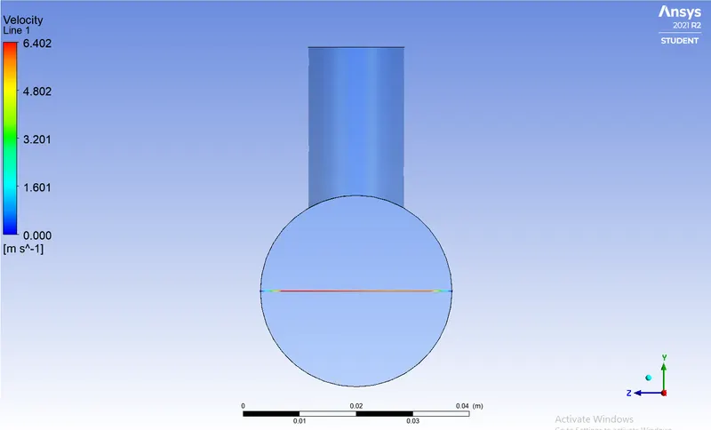
Temperature line plot across the pipe Velocity line plot across the pipe

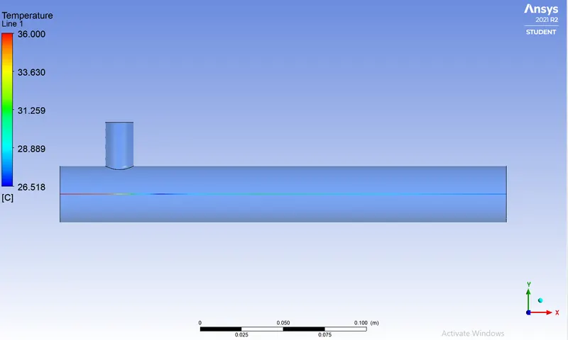
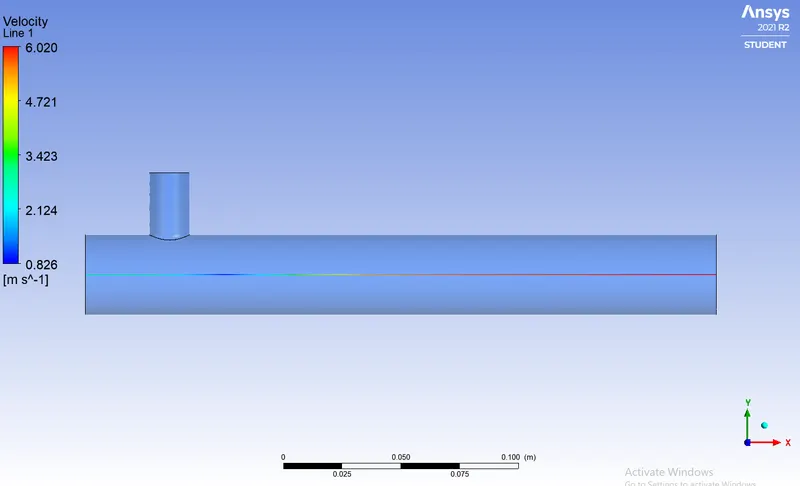
Temparature line plot along the pipe Velocity line plot along the pipe

MESH INDEPENDENT STUDY:

MESH DETAILS COMPARISION:

AIM: To show that temperature at monitor point doesn’t depend on meshing of geometry.

Here to study the mesh independent study we will consider case 4 for K-omega SST model for short Tee design. Here model of shorter length with momentum ratio of 4 is given. The inlet velocity of hot air is 3 m/s & cold air is 12 m/s. The inlet temperature of hot air is 36 degree centigrade & cold air is 19 degree centigrade.

The variation of temperature and velocity by dependence on the quality of mesh for comparing on the basis of various parameters will be studied. The residual plots, area weightage average and standard deviation temperature will be one of the parameter for this comparative observation for different meshing size and quality.

MESHING DETAILS	CASE 1 (0.015m)	CASE 2 (0.01m)	CASE 3 (0.005m)
NUMBER OF NODES	2783	2797	3142
NUMBER OF ELEMENTS	12441	12583	14247
ELEMENT SIZE	0.015m	0.01m	0.005m

Element size when was decreased from 10 mm to 5 mm. The number of nodes increased from 2797 to 3142. There was also increase in number of elements from 12583 to 14247.

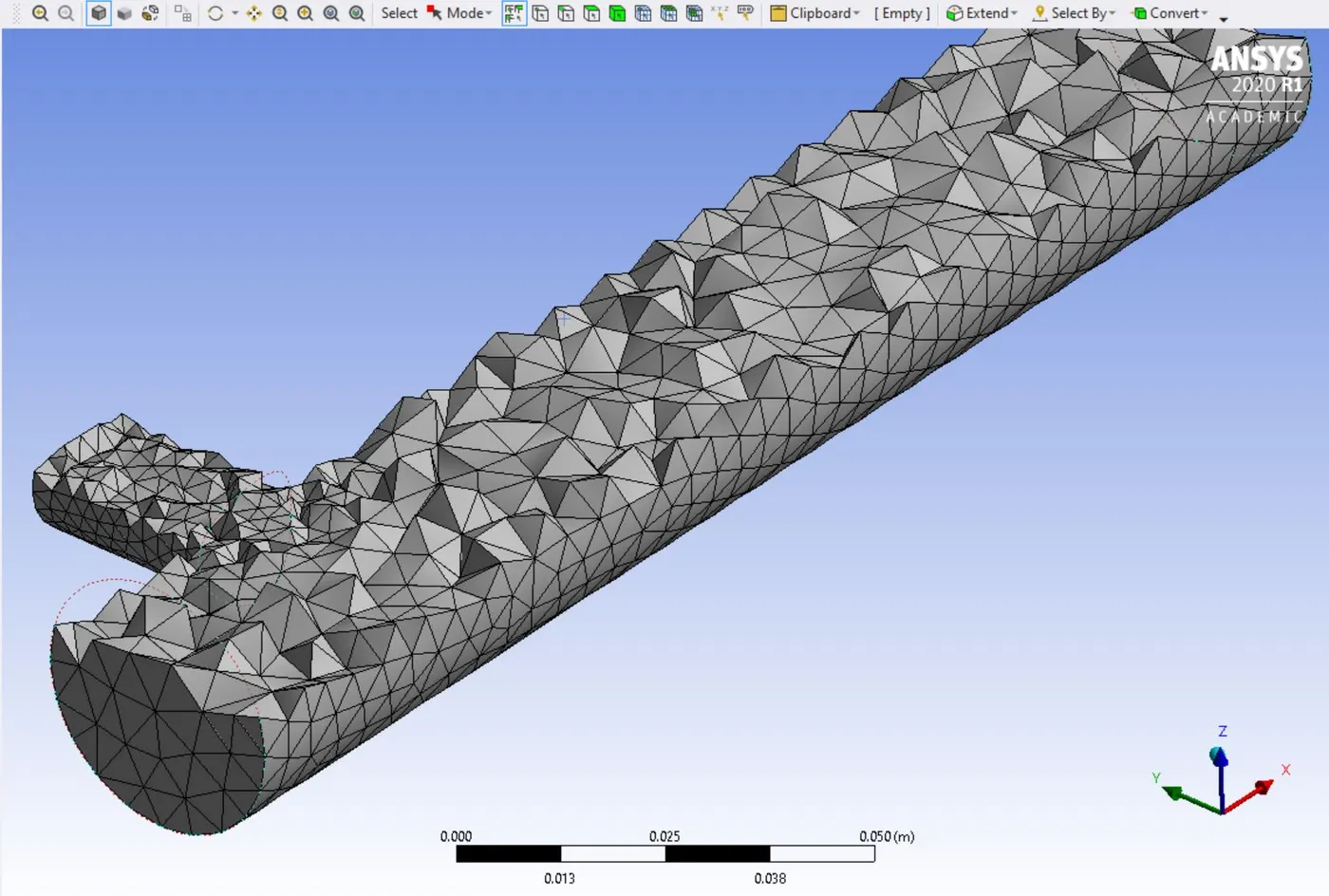
Fig: Meshing of the sectional view with tetrahedral faces for 0.01 m Element size

The elements in the below figure with 0.005m element size do look smaller in size compared to the elements of the previous fig with meshing size 0.01.

Fig: Meshing of the sectional view with tetrahedral faces for 0.005 m Element size

RESIDUE VARIABLES COMPARISION:

Below shown values of all residual variables on the plot for k-omega SST model for the elemental mesh size of 0.01m. The plot converges here after the 800+ iterations here given that the mesh size was very large comparatively for this case.

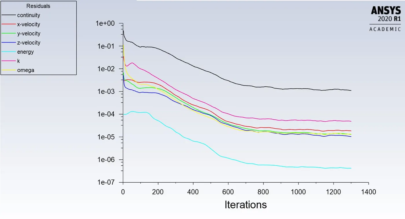
Fig: Residual plot for the mesh size of 0.01m by k-omega SST model.

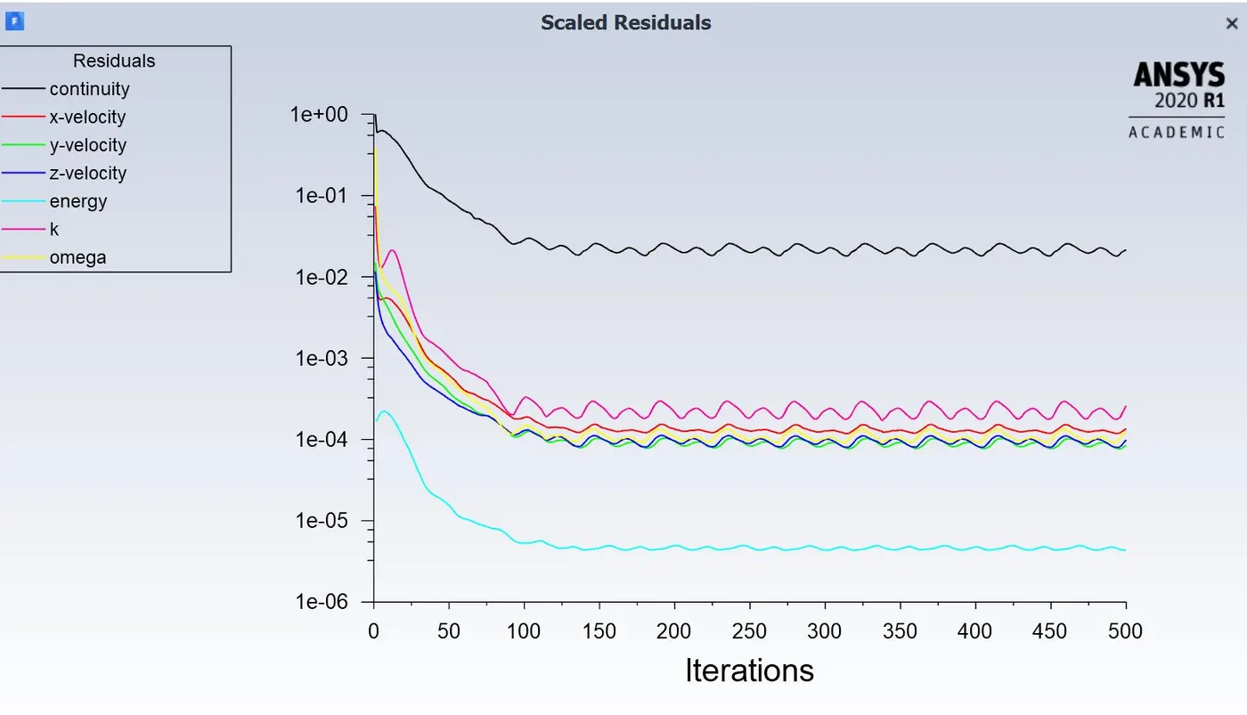
Fig: Residual pot converges more quickly here for 0.005m as compared to the bigger mesh size

Thus the number of iterations taken in the case of finer mesh is lesser as seen from the residual plots.

Area weighted average for the outlet temperature is being listed here by the plot below which is 27.55 deg C

This value for the below plot is very much similar to and almost same as the value of the other comparison case which is for 0.005m. This shows that the area weighted average temperature in both the cases are almost same.

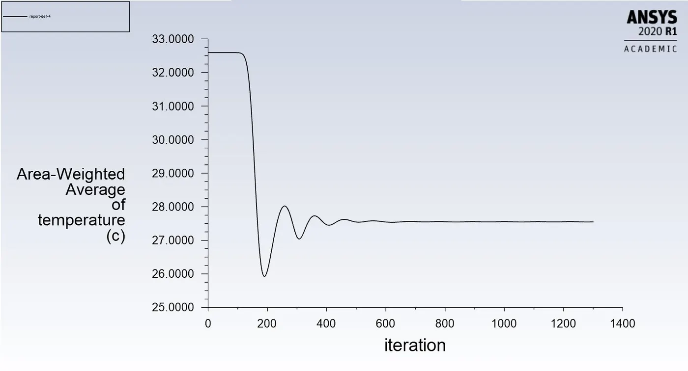
Fig: Area weighted average for outlet temperature

Also in the case of the standard deviation the value as per the below plot is 1.2572 deg C which was 1.55 deg C in the case of 0.05m mesh case which is very much near

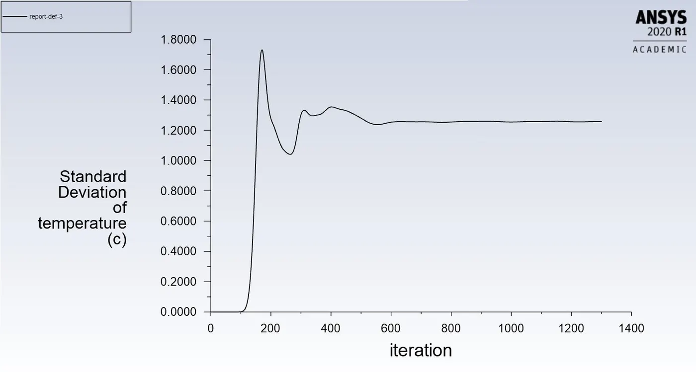
Fig: Standard deviation for the temperature at outlet for the meshing size of 0.01m

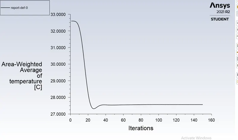
Fig: Standard deviation for the temperature at outlet for the meshing size of 0.015m

Thus it can be concluded from the comparison of plots that there is exact same outlet temperature as per the area weighted average and for standard deviation of temperature for outlet case too there is very slight change in the value of around 0.293 deg C.

This shows that even for the difference of almost twice element size there is very slight or almost no change in the outlet temperature and deviation in the temperature which do shows the mesh independency criterion and only change is the computational time for the running of simulation.

CONCLUSION:

COMPARAISION OF OUTLET TEMPERATURE FOR ALL THE CASES WITH ANALAYTICAL VALUES :

ANALAYTICAL FORMULA:-

`T_(MIX)=((m_(hot)*T_(hot))+(m_(cold)*T_(cold)))/(m_(hot)+m_(cold))`

CASES	PHYSICS	INLET VELOCITY ( m/s)		GEOMETRY TYPE	TEMPERATURE AT OUTLET(°C)	`T_(MIX)` (°C)	STANDERD DEVIATION OF TEMPERATURE(°C)
CASES	PHYSICS	HOT AIR	COLD AIR	GEOMETRY TYPE	TEMPERATURE AT OUTLET(°C)	`T_(MIX)` (°C)	STANDERD DEVIATION OF TEMPERATURE(°C)
CASE 1	k-epsilon (realizable)	3	6	SHORT TEE	30.2539°C	30.33°C	1.211075°C
CASE 2	k-omega(Shear Stress Transport (SST)	3	6	SHORT TEE	30.25°C	30.33°C	2.01°C
CASE 3	k-epsilon (realizable)	3	12	SHORT TEE	27.54°C	27.5°C	1.37455°C.
CASE 4	k-epsilon (realizable)	3	6	LONG TEE	30.2648 °C	30.33°C	1.354 °C.
CASE 5	k-epsilon (realizable)	3	12	LONG TEE	27.48819 °C	27.5°C	0.5737452 °C

Seeing the above data we can say that whether it be case of short or long geometry the velocity of inlet air plays a very big role in the outlet temperature.

The cases in which the minimum temperature inlet has the velocity of 12 m/s is the case where the temperature of inlet is around 27.5 deg C around.

Also the standard deviation in the case of longer geometry in case of momentum ratio 4 the outlet temperature is very less as compared to the rest cases. Thus apart from the cases of momentum ratio being 4 having greater efficiency we can say that the case for the longer geometry where the momentum ratio is 4 both the k-epsilon and K-omega SST model are very much effective and requires the lesser computational details for the calculations and convergence of the solution.

Also the case where the geometry is shorter and with momentum ratio of 2 and K-omega SST is the case where the standard deviation is maximum is the case which is much lesser effective than the other cases.

Thus seeing the data of results we can conclude that specifically velocity of the cooler inlet air or the momentum ratio of greater magnitude alone plays a very big role in the total resultant temperature which particularly shows the minimum deviation in the results in the case 4 & case 5 which shows the effectiveness of the results and a justified simulated comparison.

Week 1- Mixing Tee

Ship work like this
in your own course.

Talk to a career counsellor

Ship work like thisin your own course.

Talk to a career counsellor

Ship work like this
in your own course.