Week 1- Mixing Tee
Mixing Tee
Aim:-
To set up steady-state simulations for two versions of the mixing tee. One of them is longer than the other and compares the mixing effectiveness when the hot inlet temperature is 360C & the Cold inlet is at 190C.
Theory:
Computational Fluid Dynamics:
Computational Fluid Dynamics (CFD) is the analysis of fluid flows using numerical solution methods. Using CFD, you are able to analyze complex problems involving fluid-fluid, fluid-solid, or fluid-gas interaction. Engineering fields where CFD analyses are frequently used are for example aerodynamics and hydrodynamics, where quantities such as lift and drag or field properties as pressures and velocities are obtained. Fluid dynamics is involved with physical laws in the form of partial differential equations. Sophisticated CFD solvers transform these laws into algebraical equations and are able to efficiently solve these equations numerically.
CFD analyses have a great potential to save time in the design process and are therefore cheaper and faster compared to conventional testing for data acquisition. Furthermore, in real-life tests, a limited amount of quantities is measured at a time, while in a CFD analysis all desired quantities can be measured at once, and with a high resolution in space and time.
Because CFD analyses approximate a real physical solution, it should be noted that these CFD analyses cannot fully exclude physical testing procedures. For verification purposes, tests should still be performed.
NOTE:-
Simply saying CFD is a branch of fluid mechanics in which we used to track and predict the fluid flow and its reaction with surroundings using mathematical models. These mathematical models are nothing but governing equations like Navier Stokes equations(Continuity, Momentum & Mass conservation), Various Turbulence models, Heat transfer equations chemical mechanisms, etc.
A CFD analysis basically consists of the following three phases:
Pre-processing
In this phase, the problem statement is transformed into an idealized and discretized computer model. Assumptions are made concerning the type of flow to be modeled (viscous/inviscid, compressible/incompressible, steady/nonsteady). Other processes involved are mesh generation and application of initial- and boundary conditions.
Solving
The actual computations are performed by the solver, and in this solving phase, computational power is required. There are multiple solvers available, varying in efficiency and capability of solving certain physical phenomena.
Post-processing
Finally, the obtained results are visualized and analyzed in the post-processing phase. At this stage, the analyst can verify the results and conclusions can be drawn based on the obtained results. Ways of presenting the obtained results are for example static or moving pictures, graphs, or tables.
--------------------------------------------------------------------------------------------------------------------------------------
Mixing Tee:
Mixing Tees are utilized efficiently to mix two or more fluid streams into one combined stream. In this process both Mass and Heat transfer takes place. These are mainly used in HVAC applications.
In this assignment, we are going to analyze an HVAC mixing tee. Hot air is flowing through a mainstream pipe. Cold air entering through the tee, where these two hot and cold fluids mix along the pipe.
Cases:
Mesh independent study(k-epsilon)
Case 1:- element size = 0.005m
Case 2:- element size = 0.003m
Case 3:- element size = 0.002m
Compare all results from case 1,2,3 and choose right Mesh size.
suitable Turbulence model study
Case 4:- k-epsilon
Case 5:- k-omega SST
Compare all results from case 4,5 and choose the right turbulence model.
Short mixing tee (Best mesh size and Turbulence model)
Case 6:- hot inlet velocity of 3m/s, Momentum ratio of 2.
Case 7:- hot inlet velocity of 3m/s, Momentum ratio of 4.
Long mixing tee (Best mesh size and Turbulence model)
Case 8:- hot inlet velocity of 3m/s, Momentum ratio of 2
Case 9:- hot inlet velocity of 3m/s, Momentum ratio of 4.
`text(Momentum ratio) = text(velocity at cold inlet) / text(velocity at hot inlet)`
Basic Procedure for all the cases:-
1. Open ANSYS Workbench import Fluid Flow (Fluent) to the workspace.
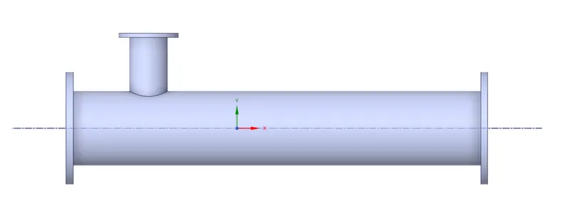
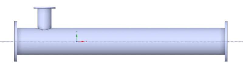
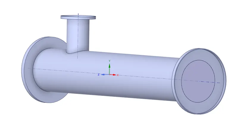
2. Double click on Geometry it will automatically redirect to space claim where we can import our Tee cad model. After importing the CAD model extract the Volume of the fluid domain using the volume extract command. this extracted fluid domain is going to represent a fluid space in physical calculations. Hide the outer shell (CAD model) and suppress it for physics. This whole process is simply called CAD clean-up.
Short Tee CAD model
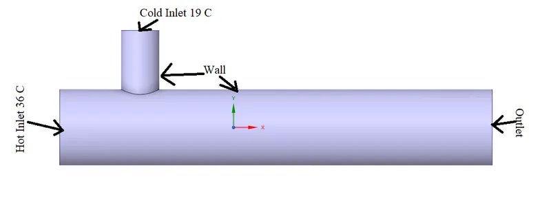
Fluid Domain
Tee + Fluid domain
Mesh:-
Update the Geometry before opening the mesh. Open mesh first verify that no external CAD model is not there except the Fluid domain. create named sections for A s follows:-
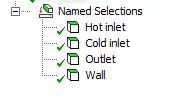
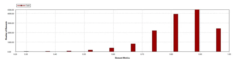
Generate mesh as per required element size and quality.
| Short Tee | ||
| Element size | Nodes | Tetrahedral elements |
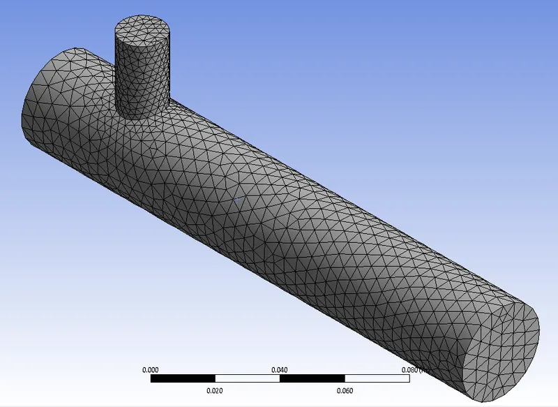
| 0.005 | 3142 | 14247 |
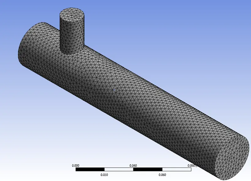
| 0.003 | 8350 | 39817 |
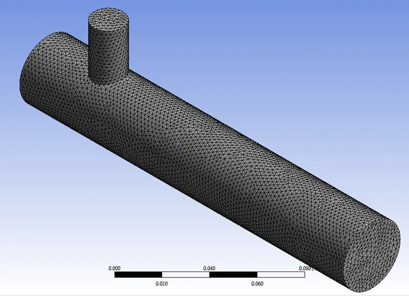
| 0.002 | 21330 | 105858 |
| Long Tee | ||
| Element size | Nodes | Tetrahedral Elements |
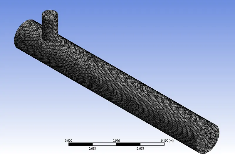
| 0.002 | 28372 | 140525 |
Short Tee element size = 0.005 m
Short Tee element size = 0.003 m
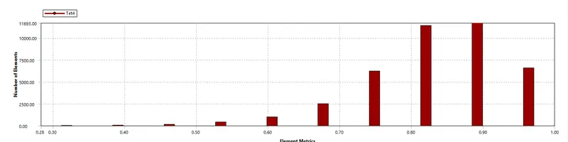
Short Tee element size = 0.002 m
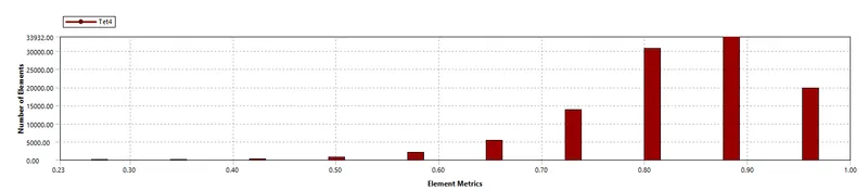
Long Tee element size = 0.002 m
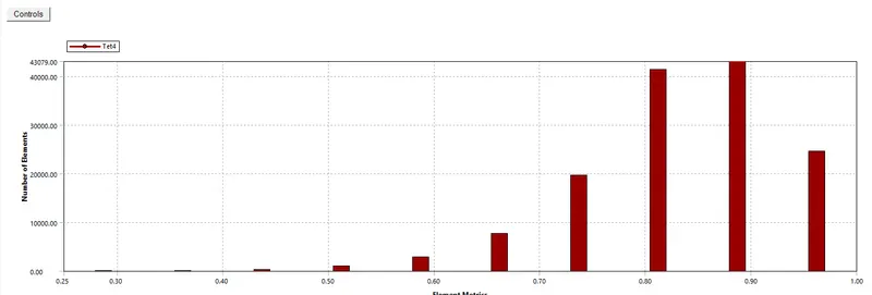
3,4. Setup & Solution.
open setup and check the file.
Setup
General settings:
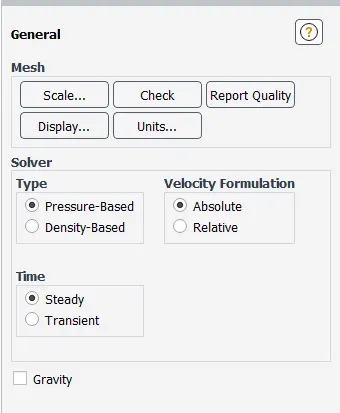
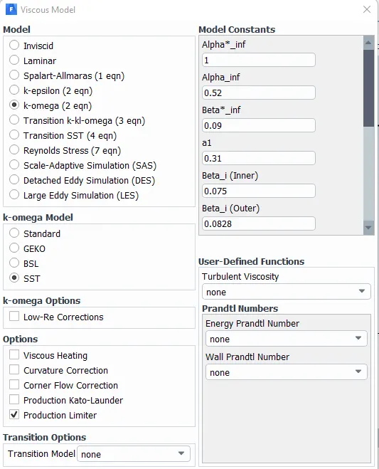
Model:-
Switch ON the energy equation.
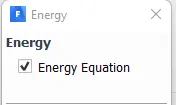
To capture turbulence we are going to use two different Viscous models
K-epsilon & K-Omega
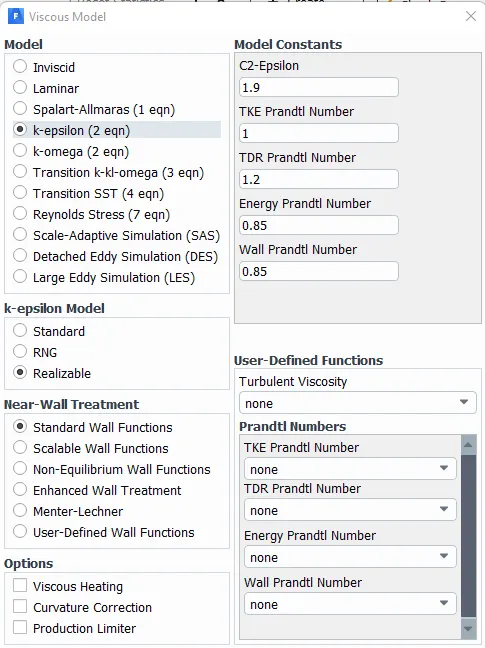
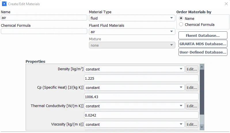
Materials:-
Air
Boundary conditions:
Cold Inlet :- Velociy inlet `T = 19 ^circ C` `V = 6 text( m/s)`
Hot inlet :- Velociy inlet `T = 36 ^circ C` `V = 3text( m/s)`
Outlet :- Pressure outlet Gauge pressure = 0 atm
Wall :- Noslip, stationary wall
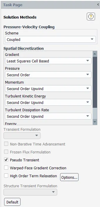
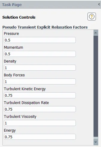
Methods & Controls:-
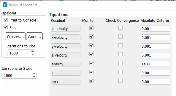
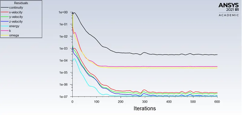
Residuals:-
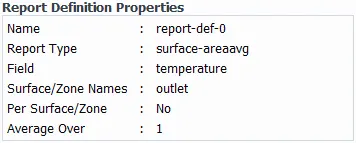
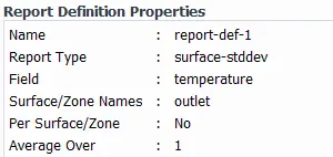
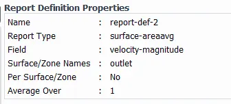
Reports:-
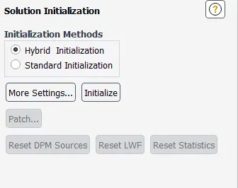
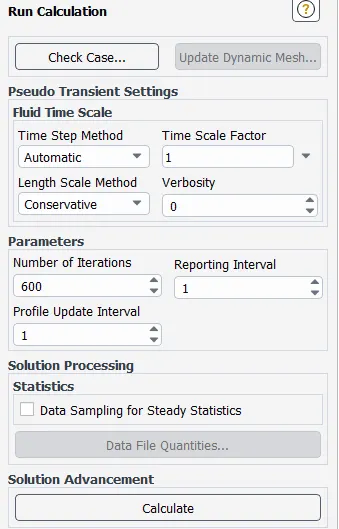
Hybrid initialization & Running Calculations:-
Results:-
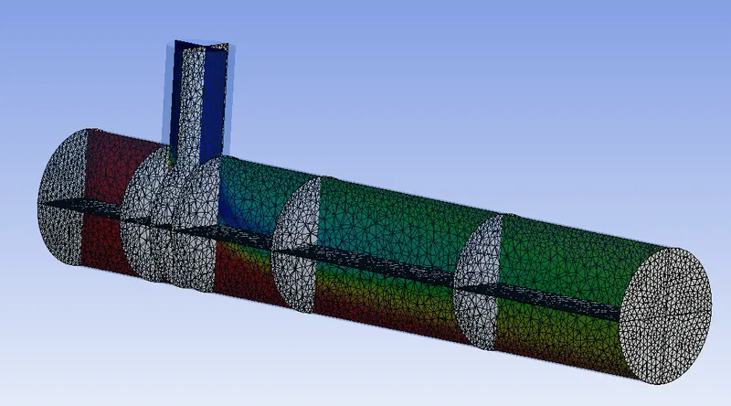
create cut plane along and across the pipe at suitable distances.
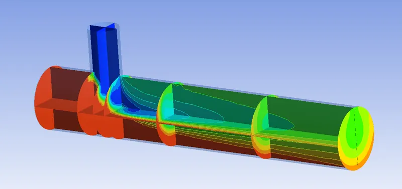
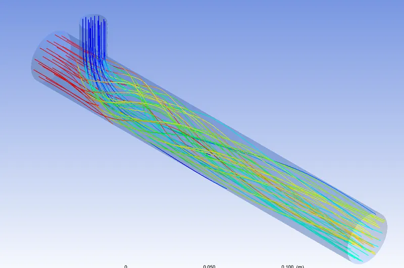
Plot Velocity and temperature contour plots
Plot Velocity and temperature line plots
Validation calculation :-
Reference Formulas:-
`T_(text(mixture)) = (m_(hot)*T_(hot)+m_(cold)*T_(cold))/(m_(hot)+m_(cold))`
`h_(text(mixture)) = (m_(hot)*h_(hot)+m_(cold)*h_(cold))/(m_(hot)+m_(cold))`
`m_(hot) = rho_(air)*A_(hot)*V_(hot)`
`m_(cold) = rho_(air)*A_(cold)*V_(cold)`
`rho_(air)= 1.225 ( kg)/m^3`
Dia of Hot inlet D_hot = 0.0338761 m
Dia of Cold inlet D_cold = 0.0169626 m
Hot inlet temperature = 36 degree Centigrade
Cold inlet temperature = 19 degree Centigrade
Code to calculate mixture temperature:
import numpy as np

# print(np.pi)

D_1 = 0.0338761 # m
D_2 = 0.0169626 # m4

Rho_air = 1.225  # kg/m3

V_1 = int(input('hot inlet velocity :-'))  # m/s
M_R = int(input('momentum ratio:-'))  # momentum ratio2
V_2 = M_R * V_1

T_hot = 36+273 # k
T_cold = 19+273 # k

A_1 = (np.pi/4)*(D_1**2) * 1e6
A_2 = (np.pi/4)*(D_2**2) * 1e6
print('Hot inlet area = ',A_1,'m2')
print('Cold inlet area = ',A_2,'m2')

m_hot = Rho_air*A_1*V_1
m_cold = Rho_air*A_2*V_2
print('Hot inlet mass flowrate = ',m_hot,'Kg/sec')
print('Cold inlet mass flowrate = ',m_cold,'Kg/sec')

T_mix =  (m_hot*T_hot + m_cold*T_cold)/(m_hot + m_cold)


print('From validation Mixture outlet temperature = ',T_mix-273, 'C')
Output:-
hot inlet velocity :-3
momentum ratio:-2
Hot inlet area =  901.315197093334 m2
Cold inlet area =  225.98245550082146 m2
Hot inlet mass flowrate =  3312.3333493180025 Kg/sec
Cold inlet mass flowrate =  1660.971047931038 Kg/sec
From validation Mixture outlet temperature =  30.322384965929984 C
---------------------------------------------------------------------------------------------------------------------------------------------
Solutions:-
Mesh independent study(k-epsilon)
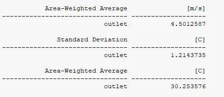
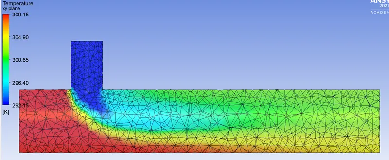
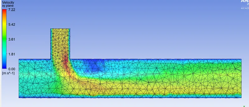
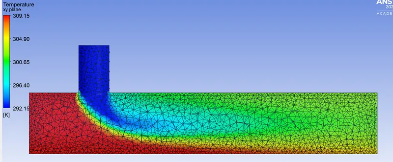
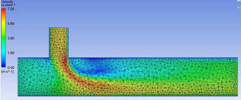
Case 1:- element size = 0.005m
Case 2:- element size = 0.003m
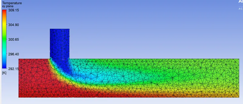
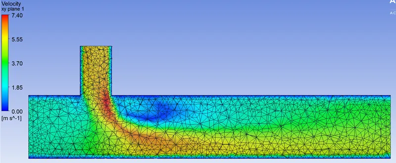
Case 3:- element size = 0.002m
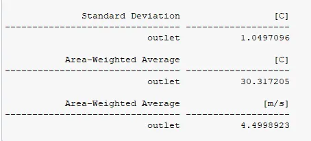
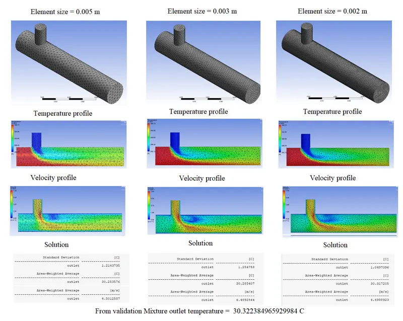
From validation Mixture outlet temperature = 30.322384965929984 C
Conclusions :
The main aim of the Mesh independent study is to find the best mesh size. Below that mesh size, there shouldn't have been any noticeable change in the final solution. In this assignment we used 3 different element sizes 0.005,0.003 & 0.002m for analysis.
From validation Mixture outlet temperature = 30.322384965929984 C
| Element size | Nodes | Tetrahedral elements |
| 0.005 | 3142 | 14247 |
| 0.003 | 8350 | 39817 |
| 0.002 | 21330 | 105858 |
| Element size (m) | outlet temperature (C) | difference(30.322384-outlet temp) |
| 0.005 | 30.253576 | 0.068808 |
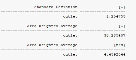
| 0.003 | 30.285407 | 0.036977 |
| 0.002 | 30.317205 | 0.005179 |
From the above tables, we can observe that for element size 0.002m the difference from actual to simulated value is 0.0051 which is very very low as compared to others. we can also observe that the number of elements is also higher for this element size. therefore computation time required for this analysis is also high. if we decrease the element size further there is a huge increase in simulation time with a small difference in solution.
Therefore, I am going to use element size = 0.002m for my next simulations.
----------------------------------------------------------------------------------------------------------------------------------------------
suitable Turbulence model study
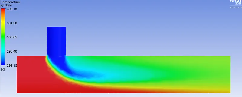
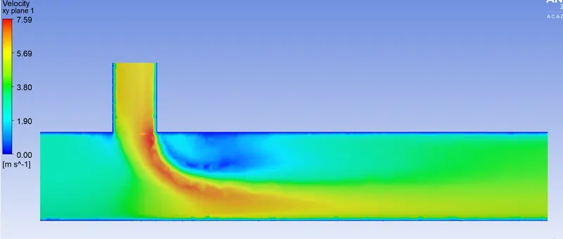
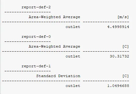
Case 4:- k-epsilon
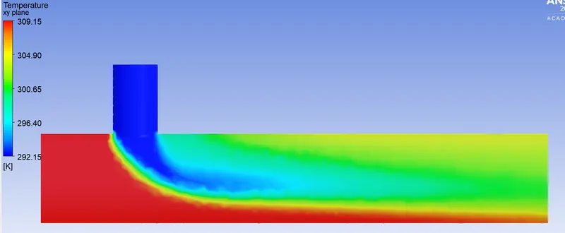
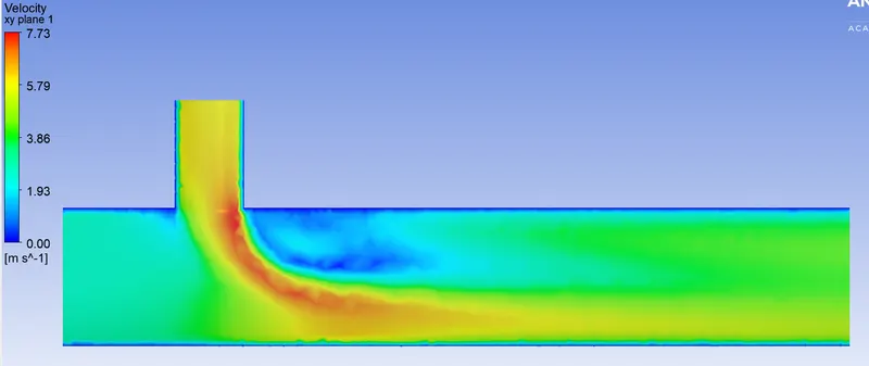
Case 5:- k-omega SST
Conclusion:-
When we compare the temperature and velocity plots from both K-epsilon and K-omega turbulence models for the same problem. where we used same we can observe that K-omega captured more turbulence than K-epsilon.
From validation Mixture outlet temperature = 30.322384965929984 C
K-epsilon temperature prediction at the outlet is = 30.31732 C
K-omega temperature prediction at the outlet is = 30.31721 C
From outlet temperature data K-epsilon predicted more accurate results than K-omega but it is not a big difference which is in order 0.0001 is neglected.
K epsilon is best suited for flow away from the wall, say free surface flow region,
whereas the k-omega model is best suited for near the wall-flow region, where the adverse pressure gradient is developed.
From the above calculations, we are going to use K-omega SST turbulence model for further analysis.
----------------------------------------------------------------------------------------------------------------------------------------------------
Short mixing tee (Best mesh size and Turbulence model)
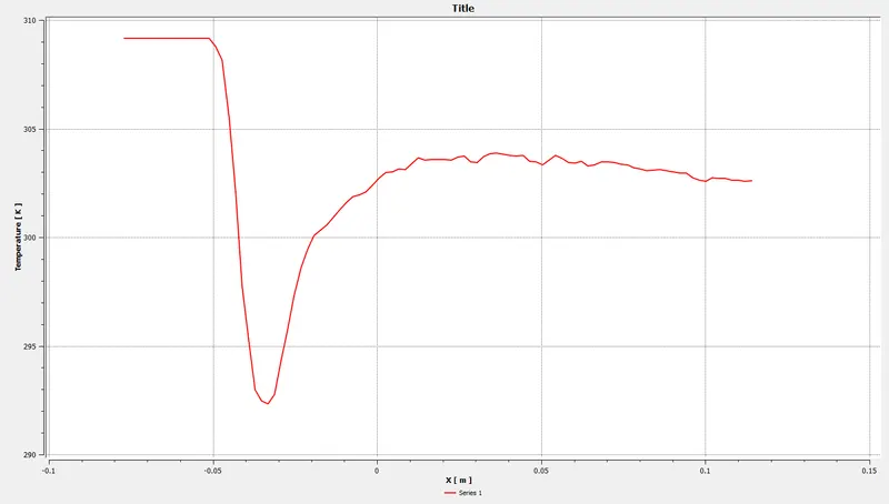
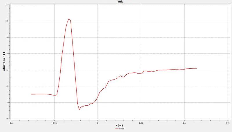
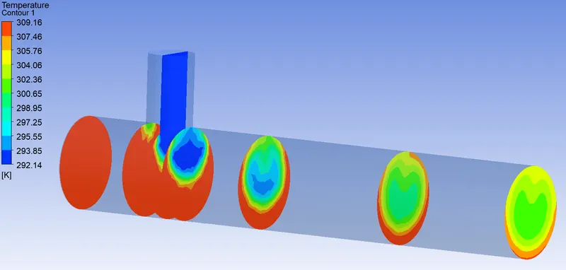
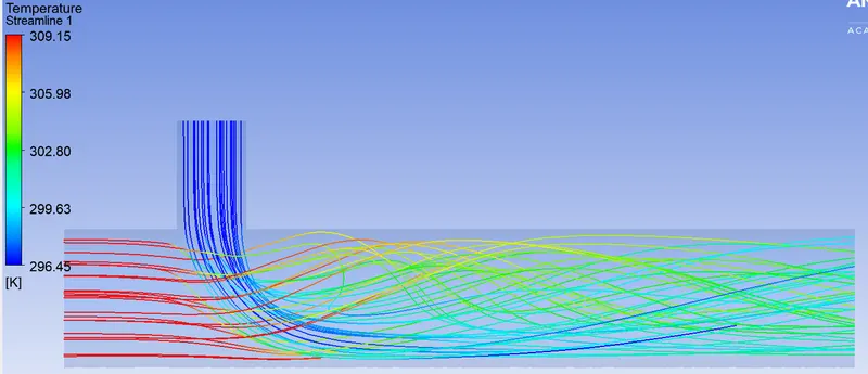
Case 6:- hot inlet velocity of 3m/s, Momentum ratio of 2.
cold inlet velocity of 6m/s
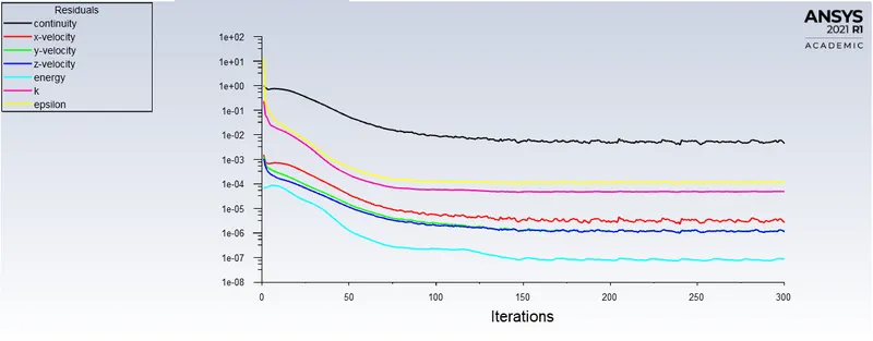
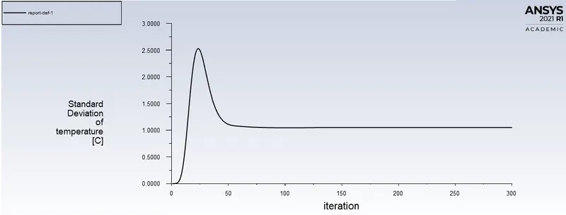
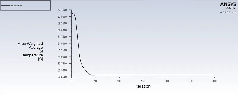
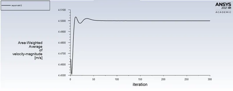
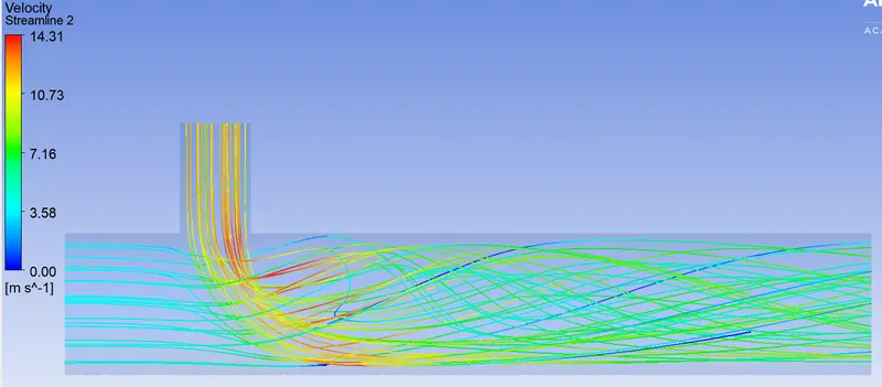
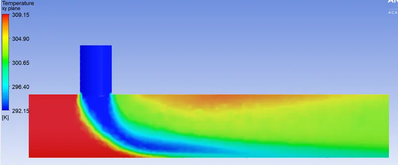
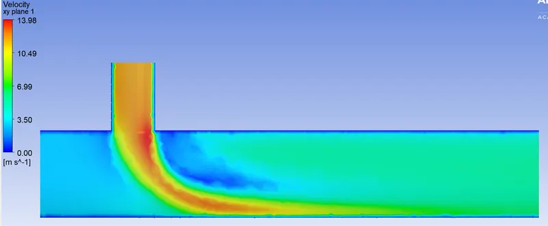
Case 7:- hot inlet velocity of 3m/s, Momentum ratio of 4.
cold inlet velocity of 12m/s
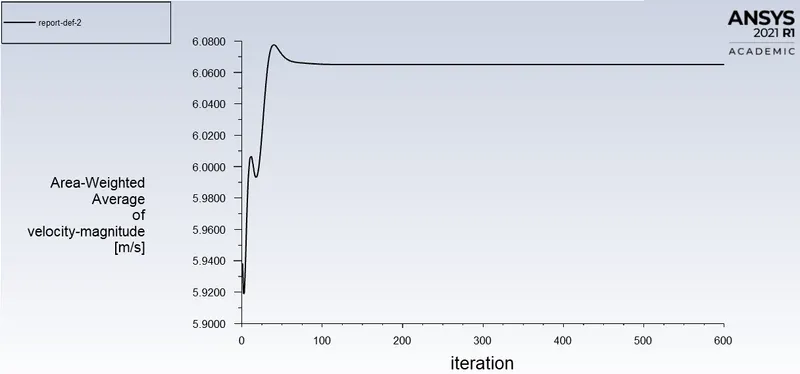
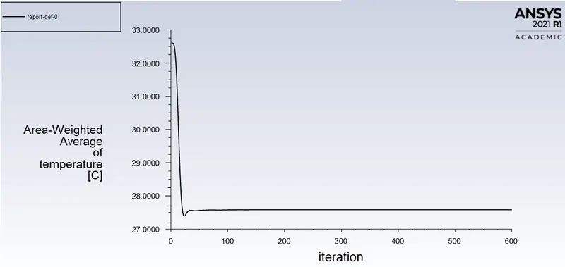
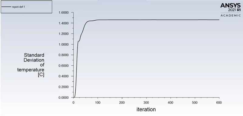
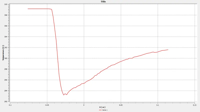
---------------------------------------------------------------------------------------------------------------------------------------------------------------
Long mixing tee (Best mesh size and Turbulence model)
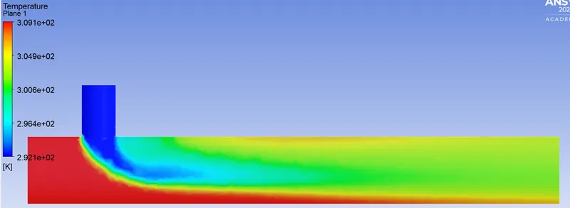
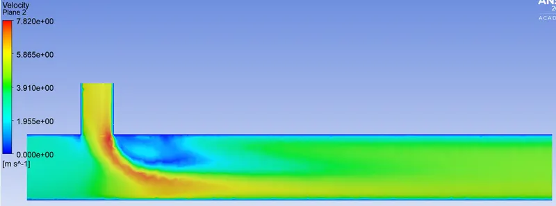
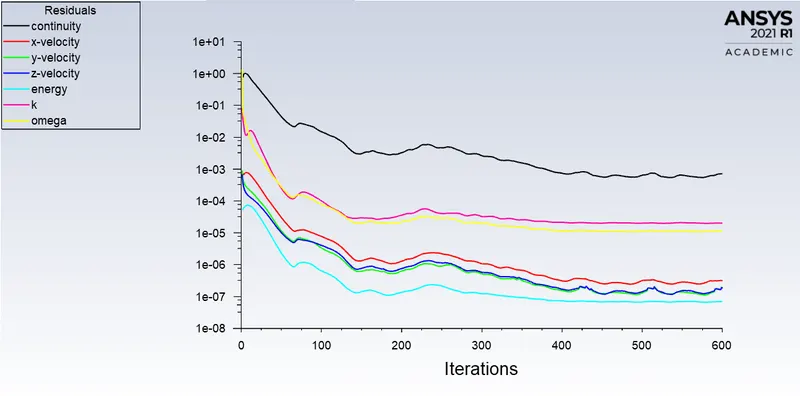
Case 8:- hot inlet velocity of 3m/s, Momentum ratio of 2
cold inlet velocity of 6m/s
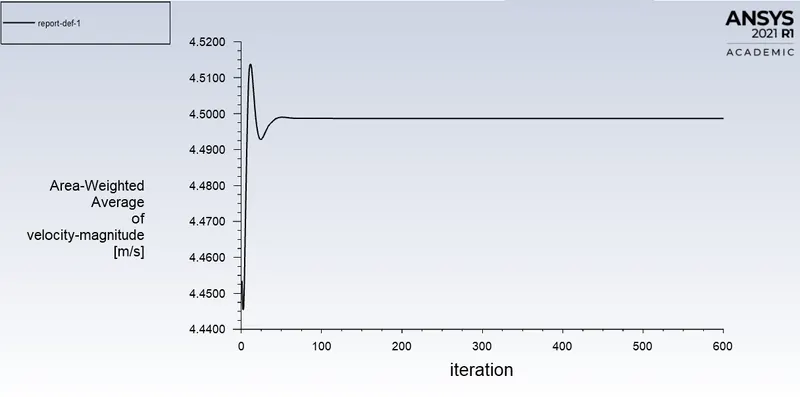
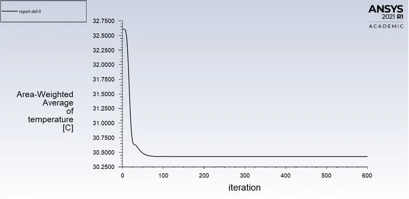
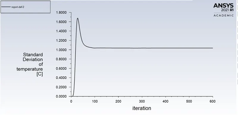
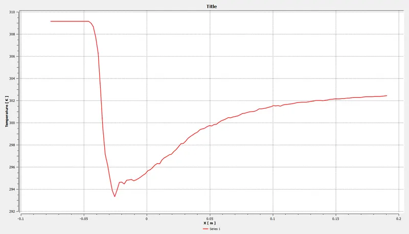
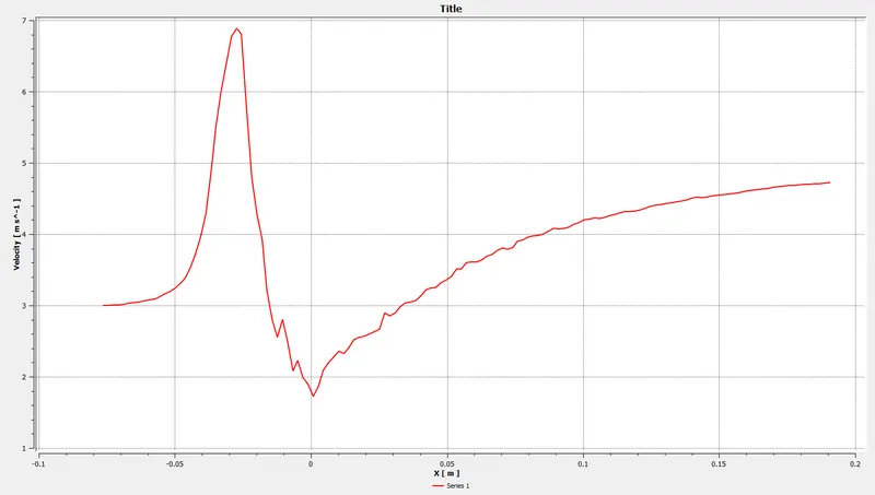
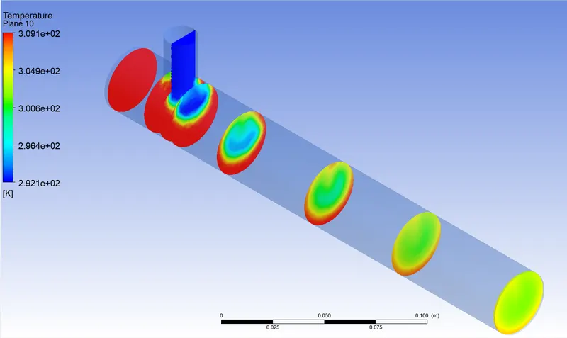
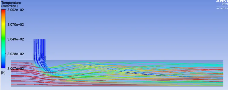
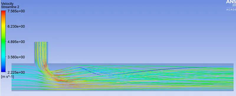
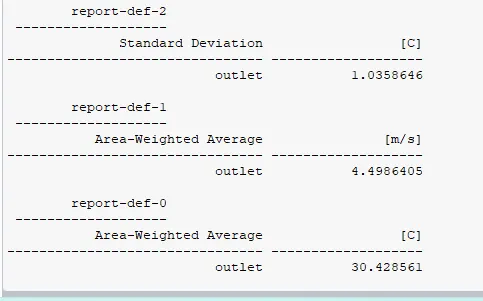
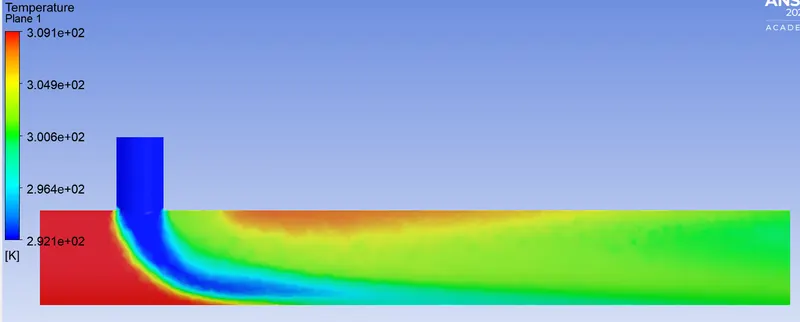
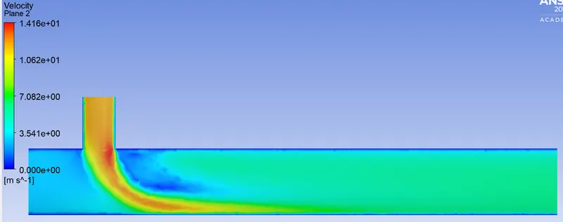
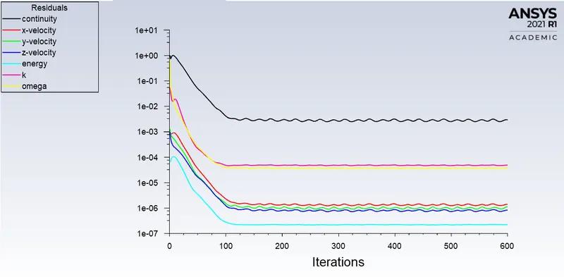
Case 9:- hot inlet velocity of 3m/s, Momentum ratio of 4.
cold inlet velocity of 12m/s
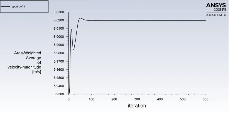
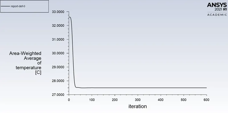
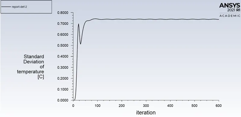
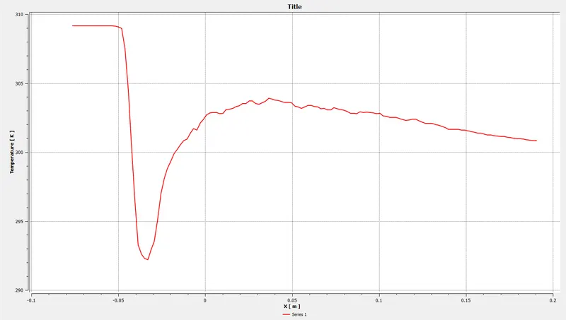
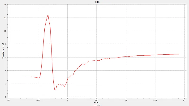
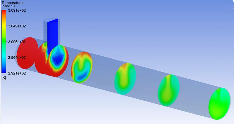
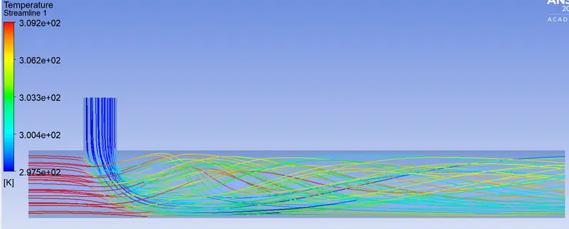
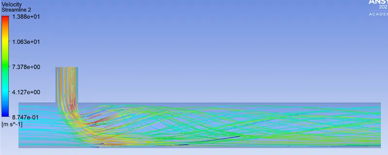
Results:-
| Result table | |||||
| Short mixing tee | |||||
|
Cell count (mesh size = 0.002m) |
The number of iterations for convergence (approx.) |
Average outlet temperature(C) |
validation outlet temperature(C) | difference(Validation-Average) | |
| Case 6:- hot inlet velocity of 3m/s, Momentum ratio of 2. | 105858 | 150 | 30.317205 | 30.322384 | 0.005179 |
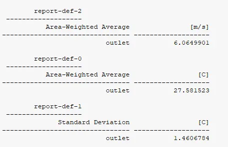
| Case 7:- hot inlet velocity of 3m/s, Momentum ratio of 4. | 105858 | 250 | 27.581523 | 27.487689 | 0.093834 |
| Long mixing tee | |||||
| Case 8:- hot inlet velocity of 3m/s, Momentum ratio of 2 | 140525 | 400 | 30.428561 | 30.322384 | 0.106177 |
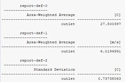
| Case 9:- hot inlet velocity of 3m/s, Momentum ratio of 4. | 140525 | 120 | 27.500397 | 27.487689 | 0.012708 |
Conclusions:-
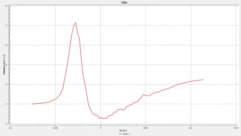
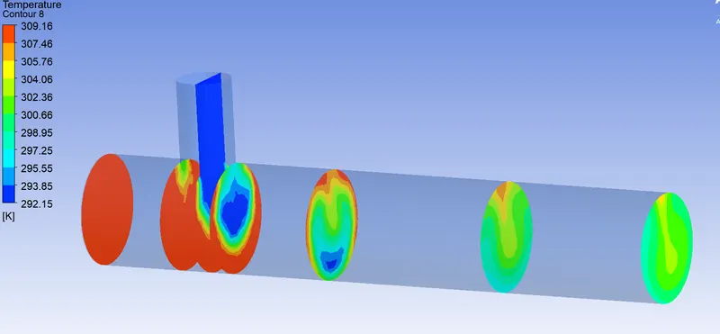
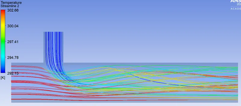
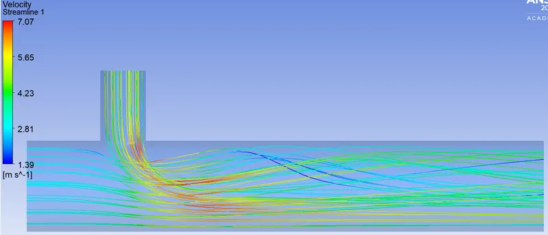
On comparison of Case, 6,7 short mixing tree mesh size 0.002m with different momentum ratios 2,4 respectively gives different Average outlet temperatures Momentum ratio (M_R) = 2 gives more colling than M_R = 4 because when MR = 2 cold inlet velocity is at 6 m/s whereas for MR = 4 cold inlet velocity is 12 m/s which double velocity as the first case. This shows that in case 7 higher velocity produces more turbulence in tee makes better mixing of hot and cold air takes place to produce chilled air than case 6. but case 6 converged quickly than case 7. increase in momentum ratio produces better results. i.e., higher momentum ratios are recommended for better output.
On comparison of Case, 7,9 short, long mixing tree with same mesh size and momentum ratios. the only difference is in the lengths of pipes. long tee is 0.075928 m longer than the short tee. from this we can observe that an increase in the length of pipe after a certain point does not produce major changes in results. from case 7,9 an increase in length of 0.0759 m produced a temperature drop of 0.08 C which is negligible. therefore short mixing tee is more suitable for this situation.
Finally, a Short mixing tee with 0.002m mesh size, K-omega SST at moment ratio 4 produces the best results.