Week 1- Mixing Tee

Aim:

To simulate the flow of air through mixing tee and understand the effect of length of pipe and momentum ratio of velocity for mixing of air by using both short pipe and long pipe.

Objective:

For this challenge, we have created two versions of the mixing tee. One of them is longer than the other.

Your job is to set up steady-state simulations to compare the mixing effectiveness when hot inlet temperature is 36⁰C & the Cold inlet is at 19⁰C.

Use the k-epsilon and k-omega SST model for the first case and based on your judgment use the more suitable model for further cases. Giving the reason for choosing a suitable model is compulsory.

1. Case 1
   • Short mixing tee with a hot inlet velocity of 3m/s.
   • Momentum ratio of 2, 4.
2. Case 2
   • Long mixing tee with a hot inlet velocity of 3m/s.
   • Momentum ratio of 2, 4.

'Momentum ratio' is defined as the ratio of velocity at the cold inlet to the velocity at the hot inlet.

Expected results:

1. Velocity and temperature contour plots on the cut planes along and across the pipe.
2. Velocity and temperature line plots along and across the length of the pipe.
3. Perform Mesh independent study for any one case.
4. Discuss the effect of length and momentum ratio on results.

Mixing Tee:

• In Industrial process engineering, "mixing" is a unit operation that involves the manipulation of a heterogeneous physical system with the intent to make it more homogeneous.
• Mixing is performed to allow the heat or mass transfer to occur between one or more streams, components or phases.
• Mixing tee is a type of mixing mechanism which utilize a specifically engineered internal geometry to efficiently mix the two fluid streams into one combined stream.
• Mixing tees are widely used in the petrochemical, HVAC indutry etc.

Problem set-up:

1. Geometry

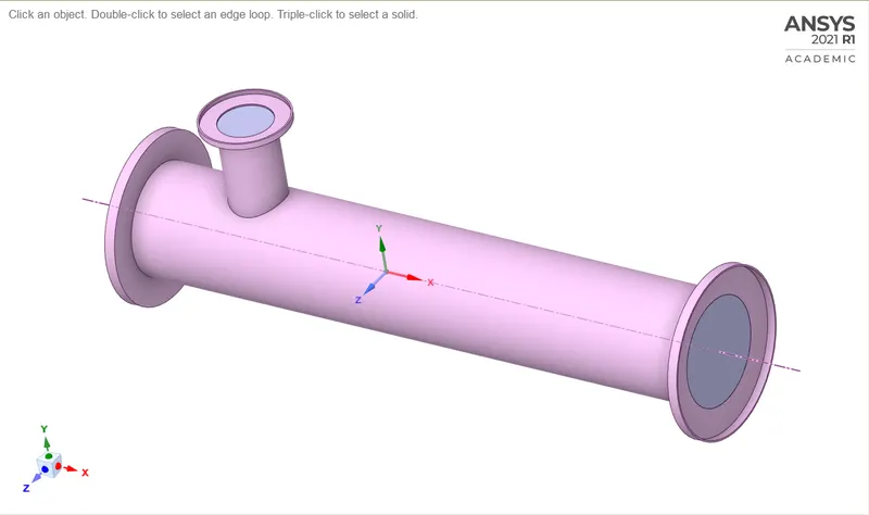
In Ansys workbench, Select the Fluid flow (Fluent) from the Analysis systems. Then click on 'import geometry' to import Mixing Tee model and right click select the 'Edit geometry on Spaceclaim' and it will redirect to Spaceclaim geometry.

2. Fluid volume Extraction

• Here, we are analyzing the mixing of two fluids only, as there is the role of a specific part hence we need to extract the volume of a tee using 'Volume extract' option in 'Prepare'.

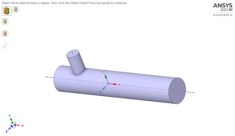
• Suppress the actual model by using the right click 'suppress for physics' option, as we don't have to make any conduction simulation in this project.

3. Meshing:

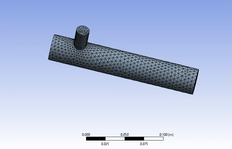
After opening the Ansys meshing, we will name the surfaces of geometry and then generate the mesh.

DEFAULT MESH SIZE - (0.010219m)

4. Setup and Solution:

• After the completion of meshing , we can move onto the setup and solution process in 'Fluent'.

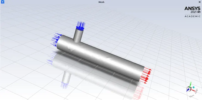
• In General, click on 'check Mesh' button to check the quality of our mesh, it prints the information in the console window.

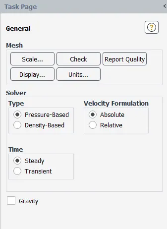
• Then we will set up the physics of the model by keeping the general setting as it is, i.e Solver type-Pressure based, Velocity formation -Absolute, Solver time- Steady.
• Next activate models and turn on the energy equations. Activating the energy equations allows the temperature-dependent problem to be solved.
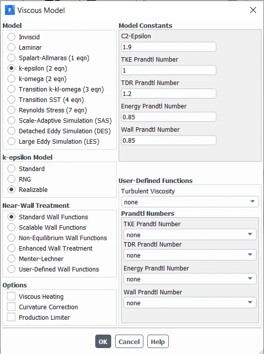
• In the viscous model, select 'K-epsilon' for our first simulation. It is a RANS based turbulence modeling. The choice of model depends on the application.

• In materials click on 'FLUENT Database' to add new material. In this case, our working fluid is air So, we can keep the default material and type as Fluid.
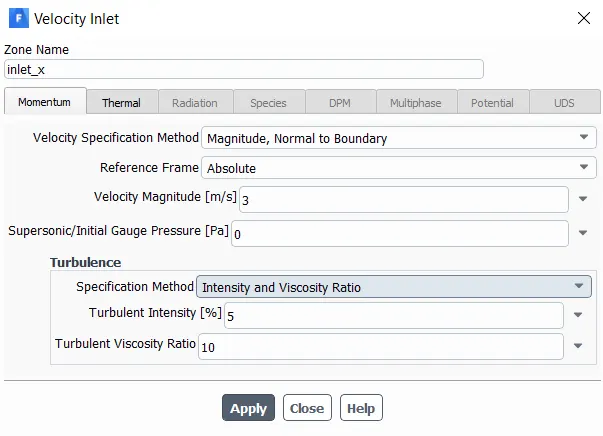
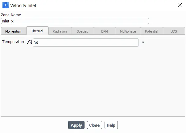
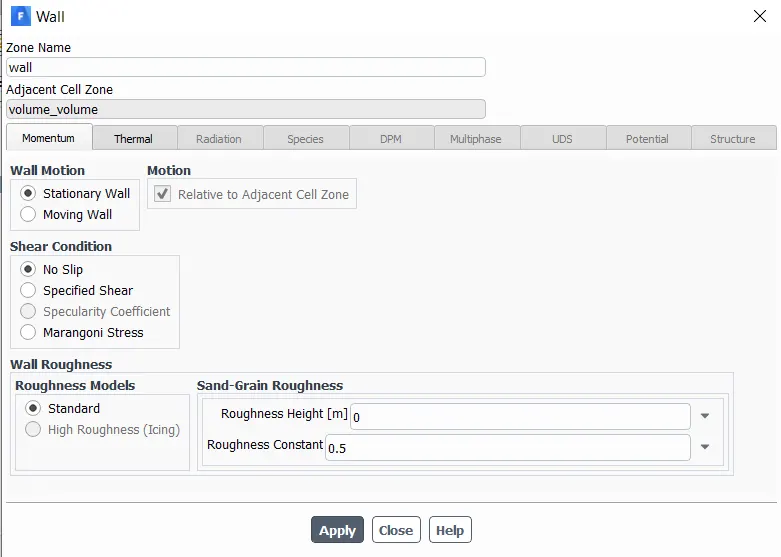
• In 'Boundary condition' click on inlet_x and set the parameter velocity as 3m/s and temperature as 36 degree Celsius. For inlet_y velocity as 12 or 6 m/s based on the momentum ratio for the case and temperature as 19 degree celsius.

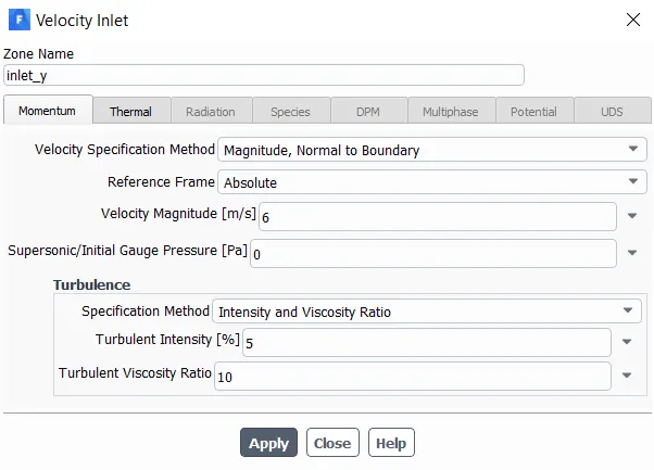
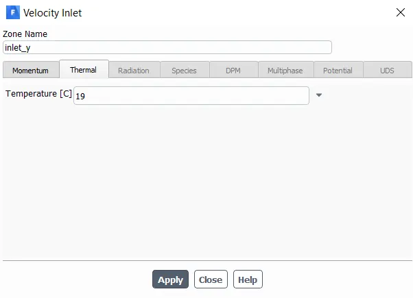
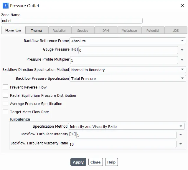
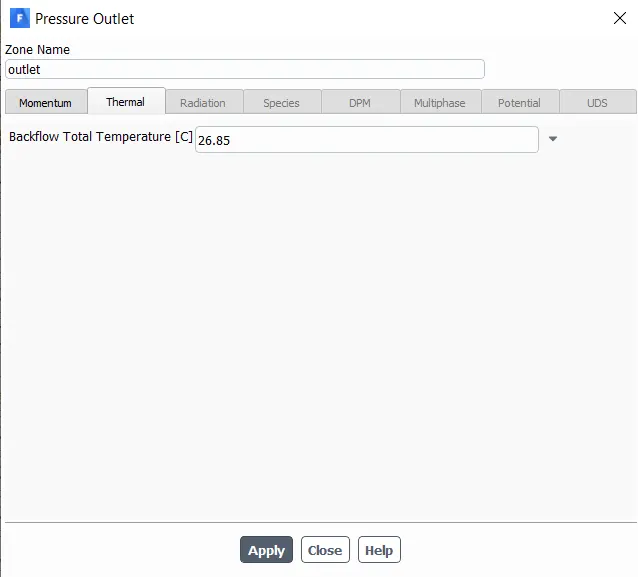
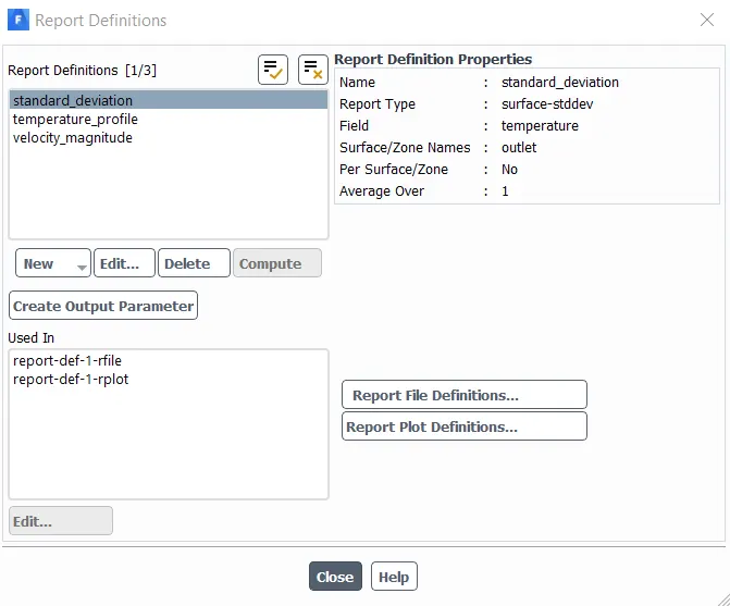
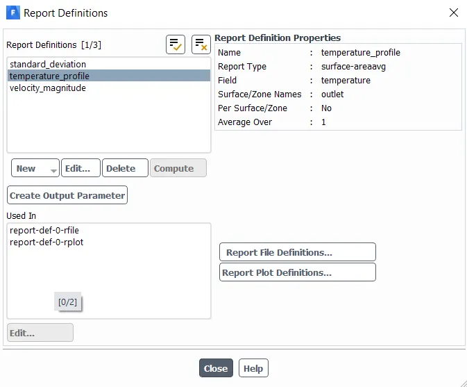
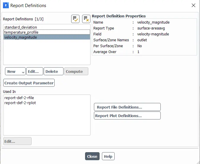
• In Solution, select 'Definitions' from the 'Reports' and select 'New' for surface report monitoring. Select Area weighted average for temperature and then for velocity and enable "report file"and "report plot".

• The final step is to initialize, Select Hybrid initilization and check the console window for the initialization done.

• Enter the no.of iterations and press 'Calculate'. After the calculation is done we will get the required plots and information.
• We can see the results as contour plots , line plots in 'CFD post' processing.

Comparison of K-epsilon and K-omega turbulence models

PLOTS:

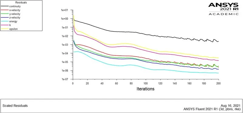
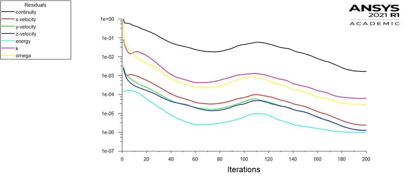
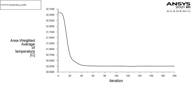
1. K-epsilon: CONVERGENCE PLOT

CONTOUR PLOTS:

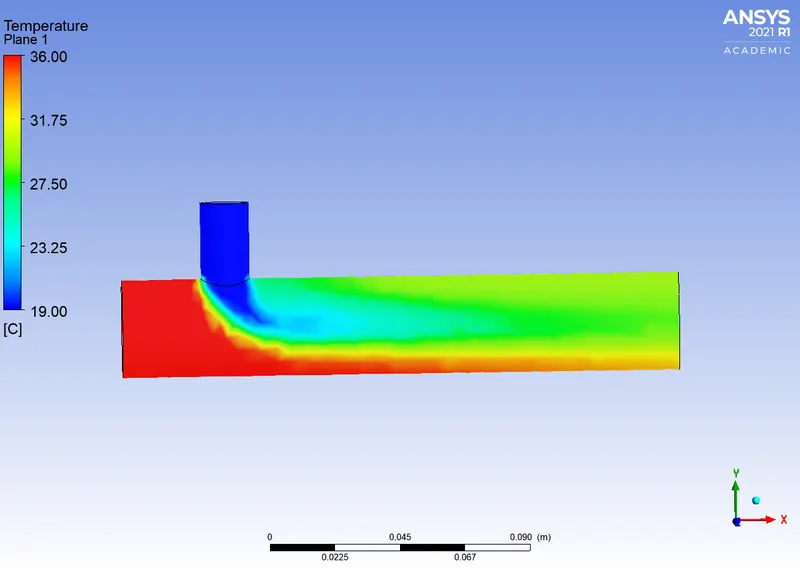
Temperature Contour

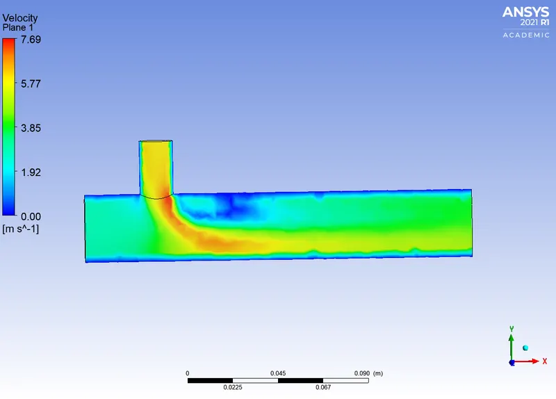
Velocity Contour

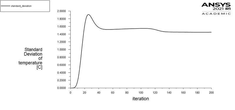
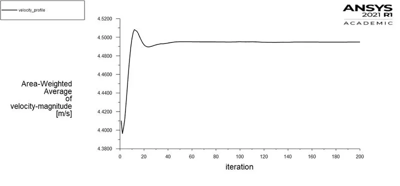
2. K-omega SST: CONVERGENCE PLOT

CONTOUR PLOTS:

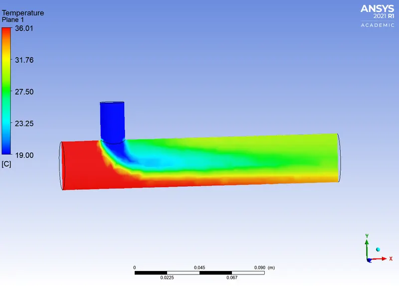
Temperature Contour

Velocity Contour

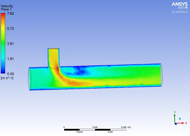
From the above contour plots, we can see the flow differences in both the models. Let us understand what's the difference between them in the following context.

K-epsilon:

• It is a RANS based turbulence model which is the most commonly used model in CFD to simulate the mean flow characteristics for turbulent flow conditions. It is a two-equation model that gives a description of turbulence by means of two transport equation (PDE's).
• The first transport variable is turbulent kinetic energy and the second transport variable is the rate of dissipation of turbulent kinetic energy.
• K-epsilon focuses on the mechanism that affects the turbulent kinetic energy.

K-Omega SST:

• K-Omega SST (Shear stress Transport) is a two-equation eddy viscosity model that is used for many aerodynamics applications. It is a hybrid model combining the wilcox omega and K-epsilon models.
• A blending function activates the wilcox model near the wall and K-epsilon in the free stream. This ensures that the appropriate model is utilized through the flow field.

Difference:

• K-omega model is well suited for simulation flow in the viscous sub-layer. On the other hand, K-epsilon is ideal for predicting flow in the regions away from the walls.
• K-omega model exhibits less sensitivity to the free stream conditions than any other turbulence models.

In this particular case, we are not dealing with the walls, therefore we are going to use the K-epsilon turbulence model for further simulation.

CASE 1(a):

Short Mixing Tee:

• Inlet velocity (hot air) - 3m/s
• Momentum ratio - 2

Convergence Plot

• Here, we have run the simulation for 200 iterations but the solution is converging at around 140 iterations.

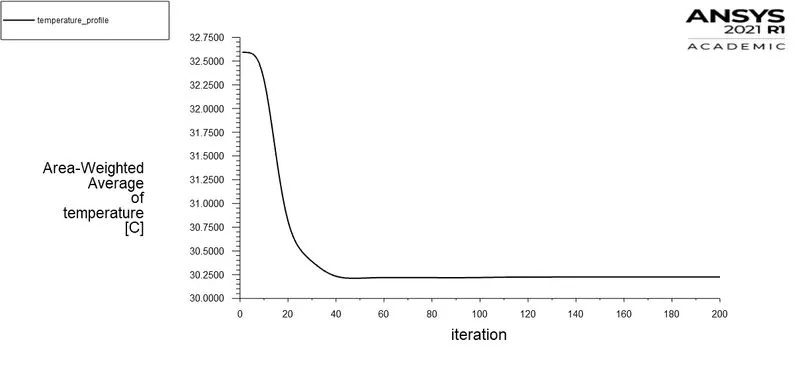
Area weighted average outlet temperature

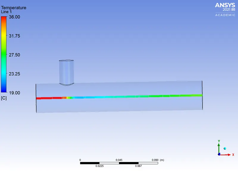
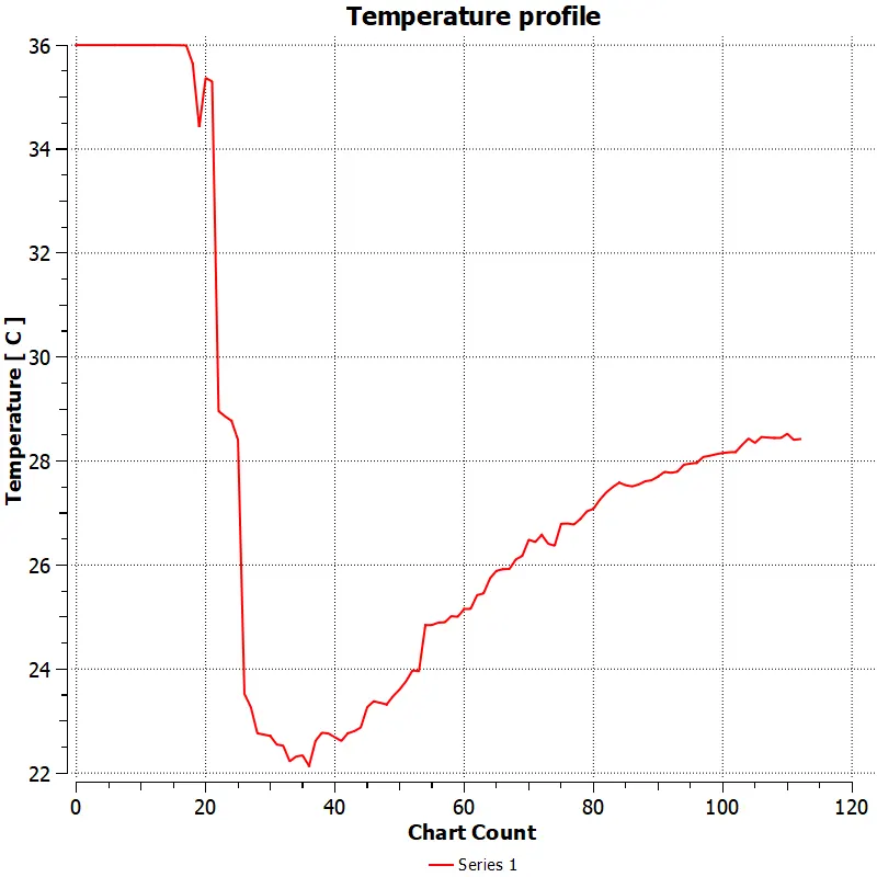
• The average temperature at the outlet is 30.225°C.

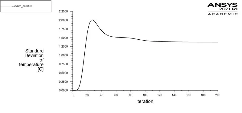
Standard Deviation

• The standard Deviation of temperature is 1.3736°C which is low. Therefore, the effectiveness of mixing is good.

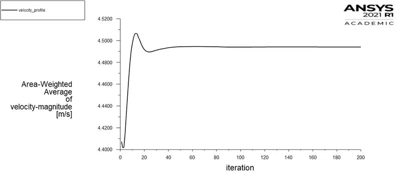
Area weighted average velocity magnitude

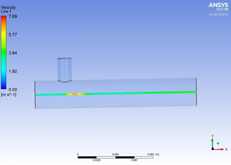
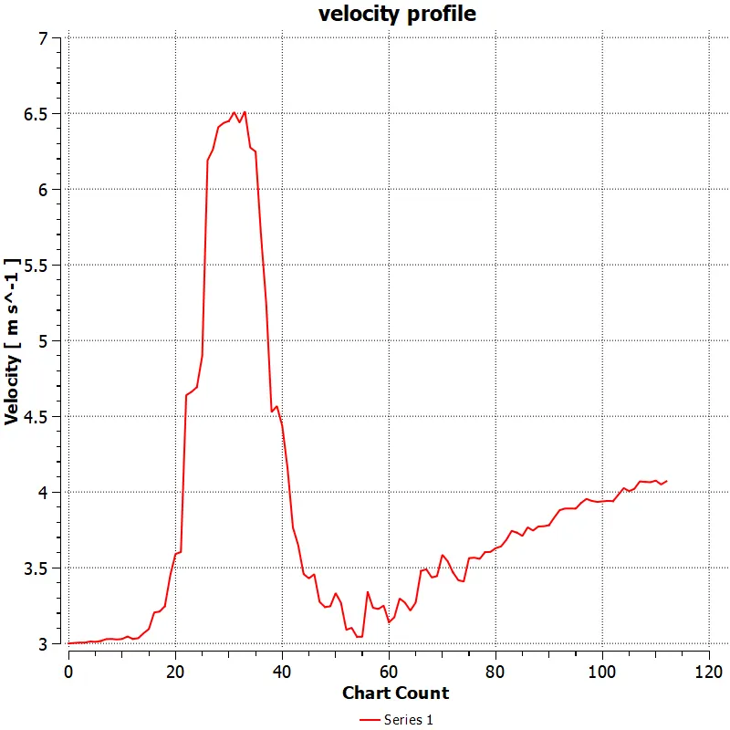
• The average velocity at the outlet is 4.5 m/s

Temperature Contour

Velocity Contour

Temperature Line Plot

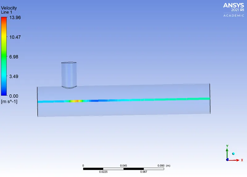
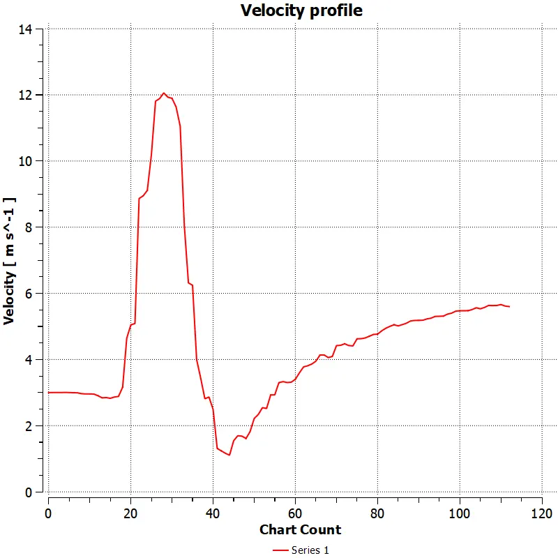
Velocity Line Plot

CASE 1(b):

Short Mixing Tee:

• Inlet velocity (hot air)- 3m/s
• Momentum ratio - 4

Convergence Plot

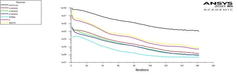
• The solution is converging at 162 iterations .

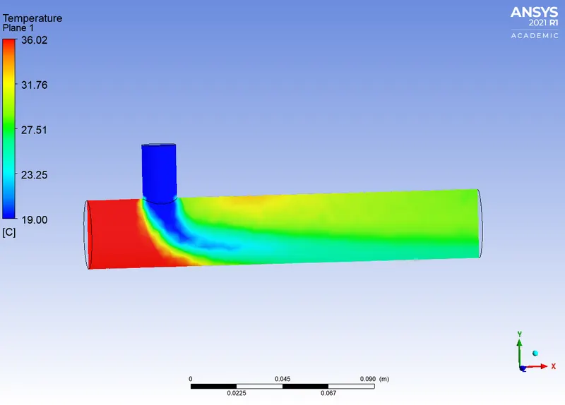
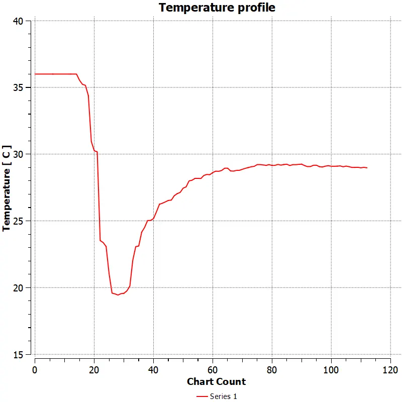
Area weighted average outlet temperature

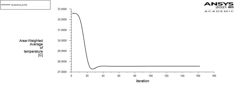
• The average temperature at the outlet is 27.555°C.

Standard Deviation

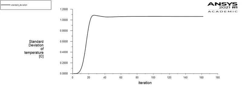
• The standard Deviation of temperature is 1.0637°C which is low. Therefore, the effectiveness of mixing is good.

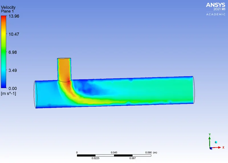
Area weighted average velocity magnitude

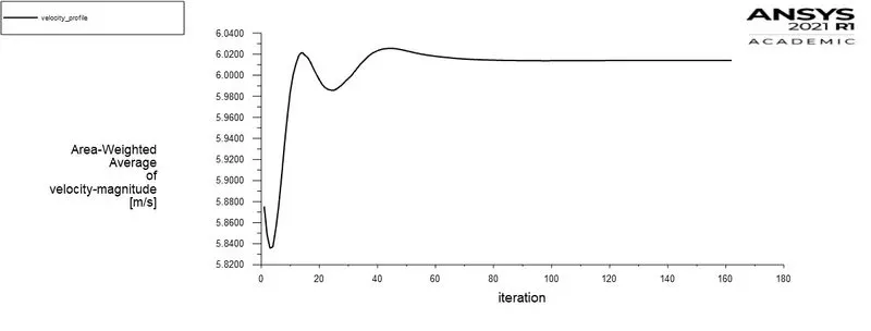
• The average velocity at the outlet is 6.014 m/s.

Temperature Contour

Velocity Contour

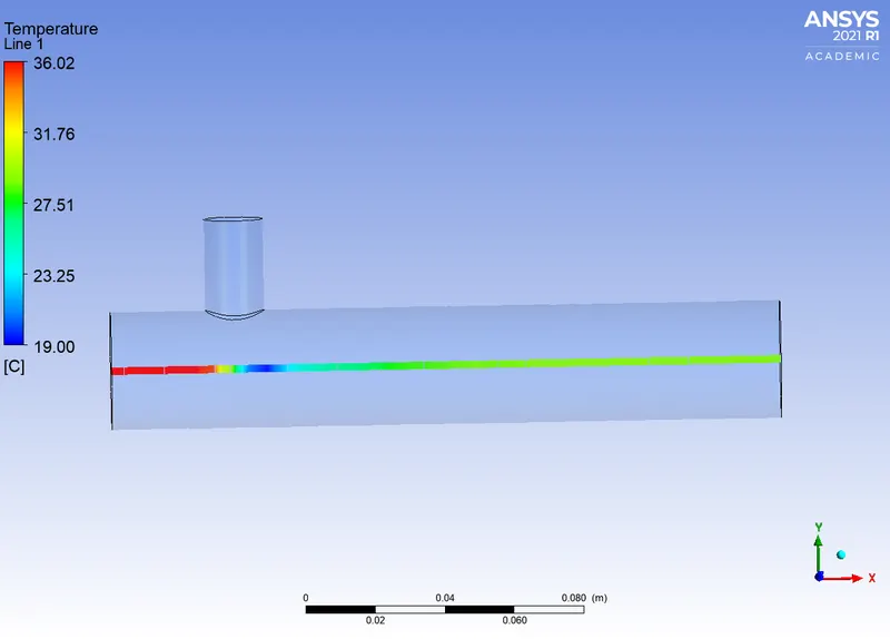
Temperature Line Plot

Velocity Line Plot

CASE 2(a):

Long Mixing Tee:

• Inlet velocity (hot air) - 3m/s
• Momentum ratio - 2

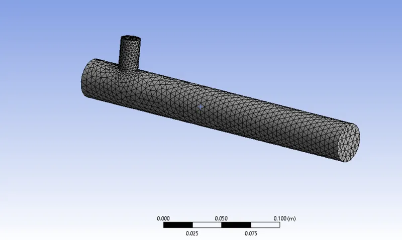
Mesh:

DEFAULT MESH SIZE - (0.013853m)

Convergence Plot

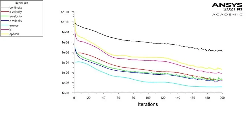
• We have run the simulation for 200 iterations and found out that the solution is converging at around 168 iterations.

Area weighted average outlet temperature

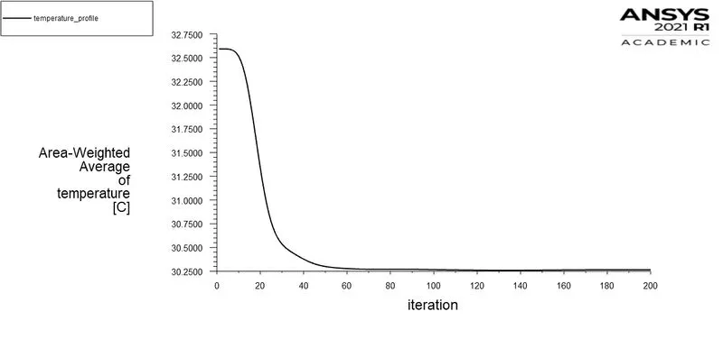
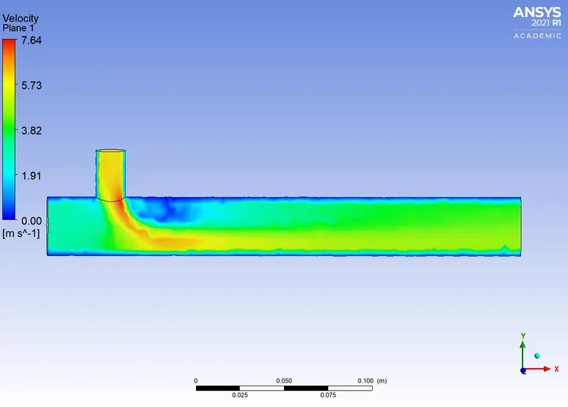
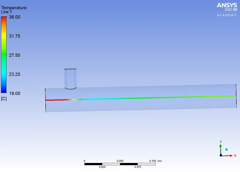
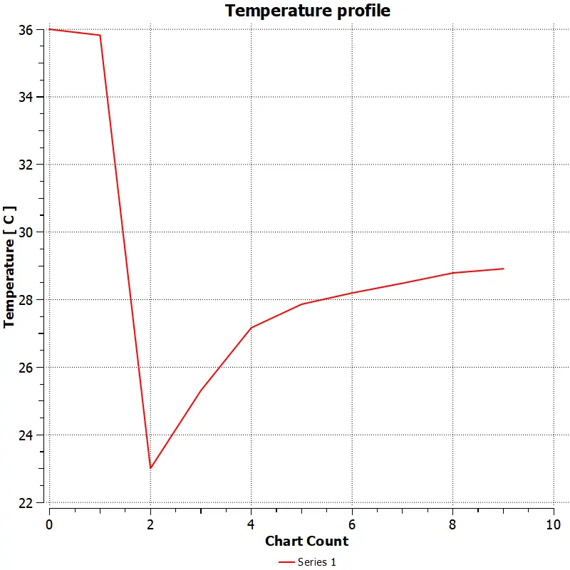
• The average temperature at the outlet is 30.2646°C.

Standard Deviation

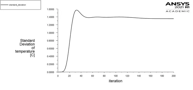
• The standard deviation of temperature is 1.3538°C which is low. Thus, the effectiveness of mixing is good.

Area weighted average velocity magnitude

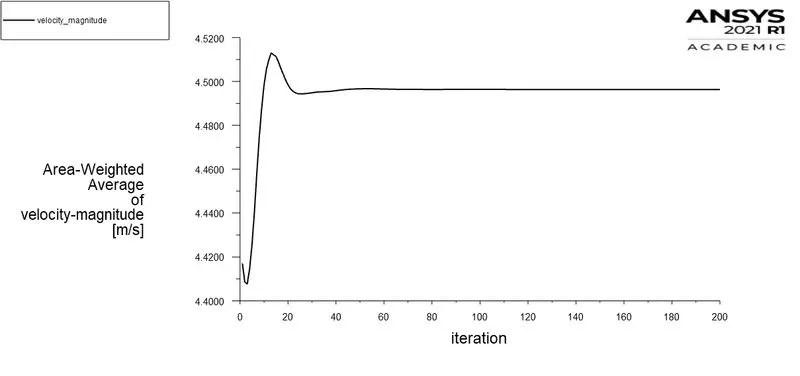
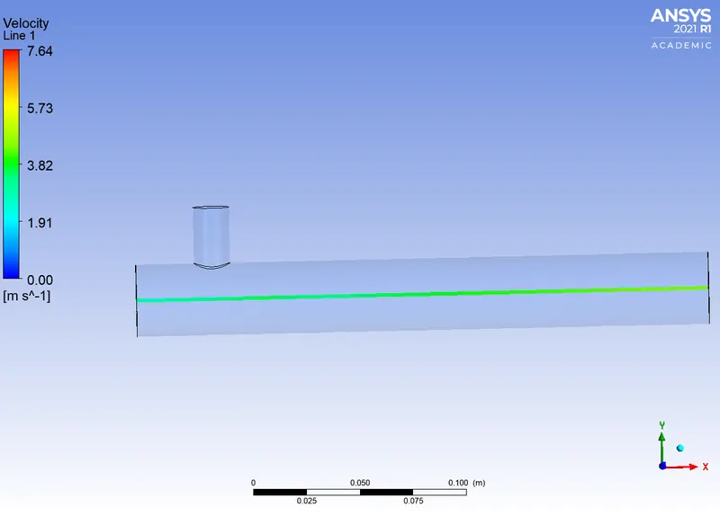
• The average velocity at the outlet is 4.4962 m/s.

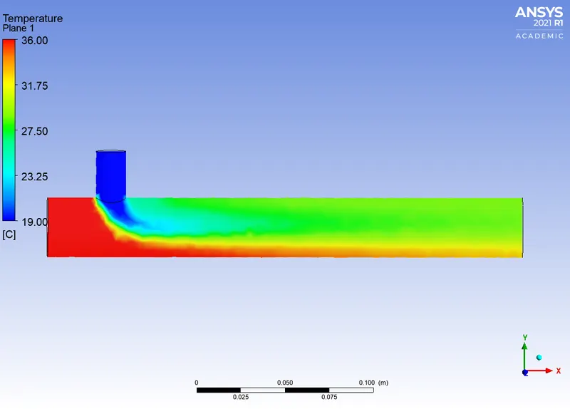
Temperature Contour

Velocity Contour

Temperature Line Plot

Velocity Line Plot

CASE 2(b):

Long Mixing Tee:

• Inlet velocity (hot air) - 3m/s
• Momentum ratio - 4

Convergence Plot

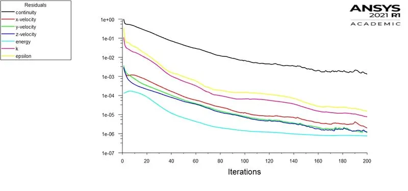
• We have run the simulation for 200 iterations and found out that the solution is converging at around 185 iterations.

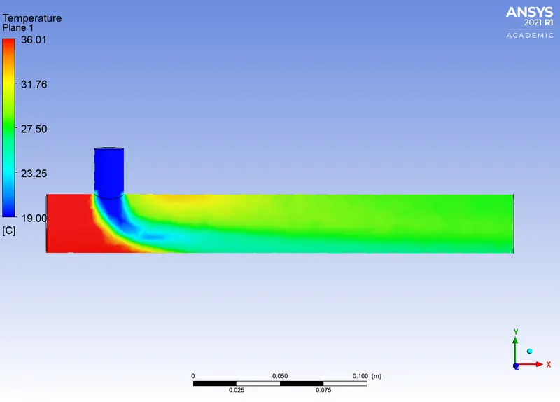
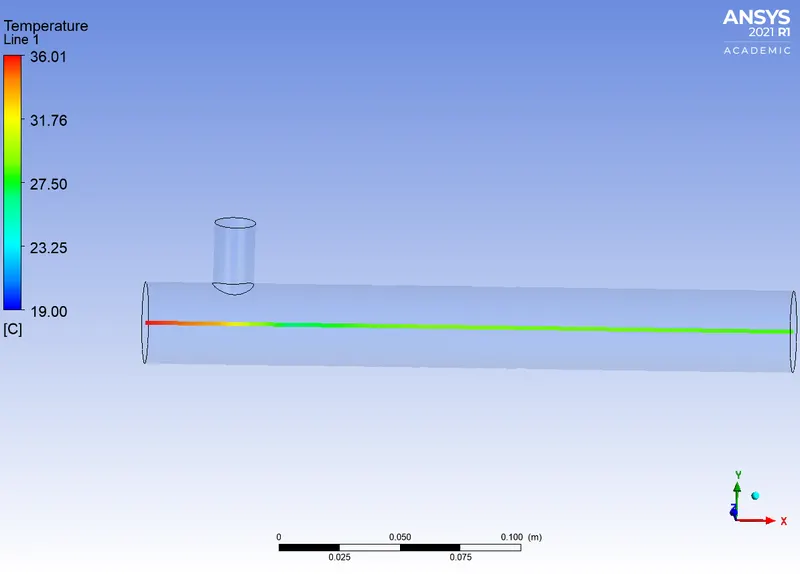
Area weighted average outlet temperature

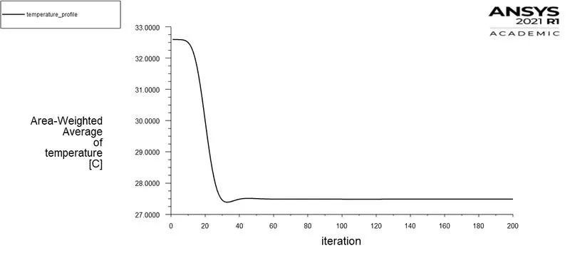
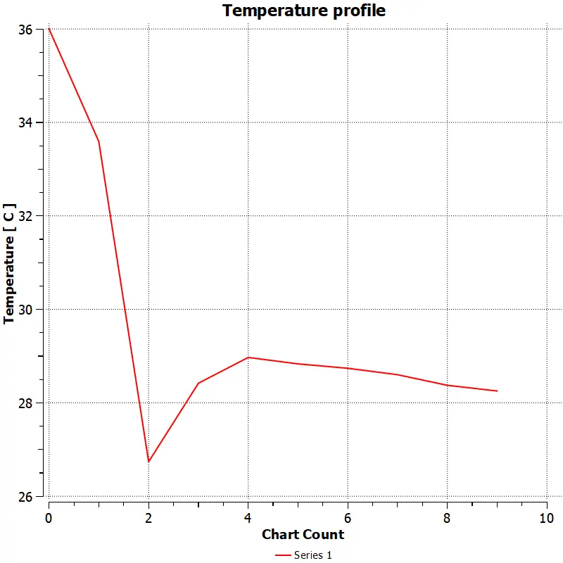
• The average temperature at the outlet is 27.4883°C.

Standard Deviation

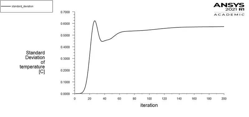
• The standard deviation of temperature is 0.5727°C which is low. Thus, the effectiveness of mixing is good.

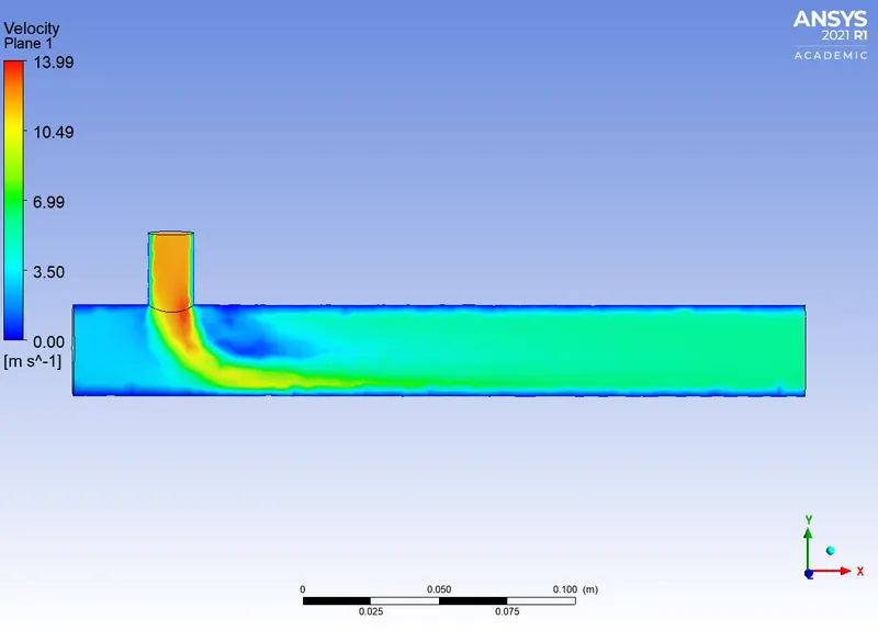
Area weighted average velocity magnitude

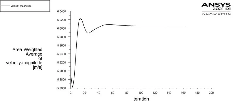
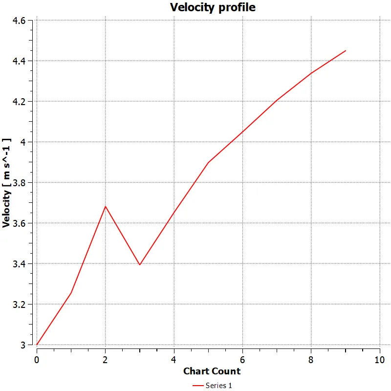
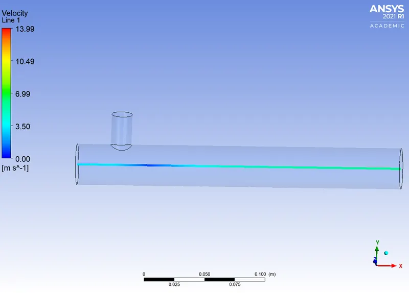
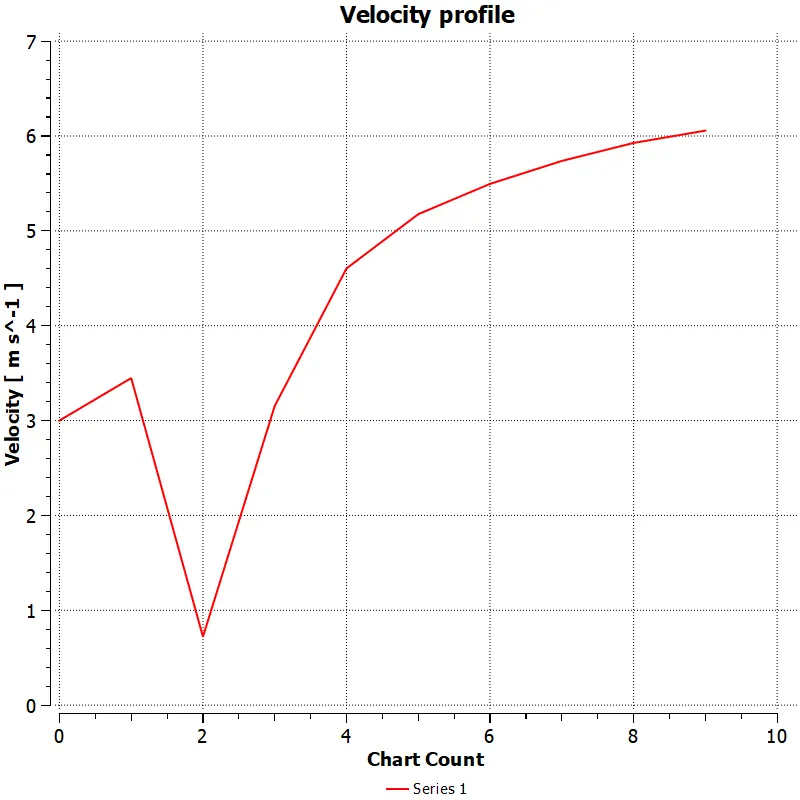
• The average velocity at the outlet is 6.0048 m/s.

Temperature Contour

Velocity Contour

Temperature Line Plot

Velocity Line Plot

Mesh Quality check using Element quality:

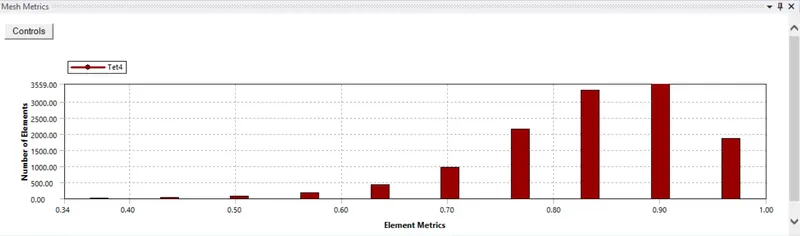
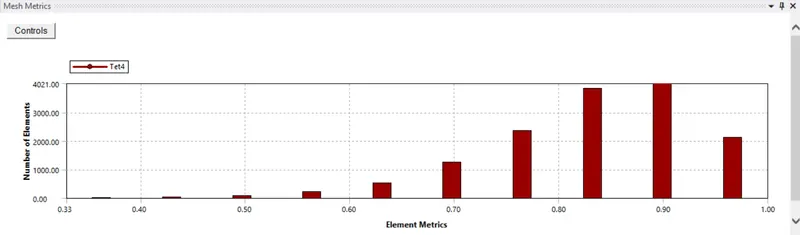
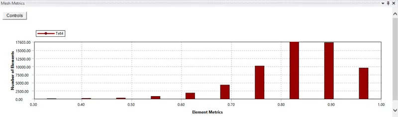
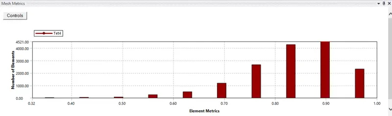
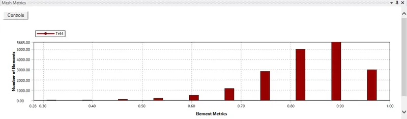
• In order to check the mesh quality, we can select the 'quality' option in dialogue box of meshing and then select 'Mesh metric' from which select the 'Element Quality' is selected. After that the bar graph shows the quality of elements below the main screen.
• Which describes that the most of the elements should be greater than 0.5 for good quality meshing.

Element Quality for different size of meshing (Short Tee):

1. DEFAULT MESH SIZE - (0.010219m)

2. MESH SIZE - (0.005m)

3. MESH SIZE - (0.0025m)

Element Quality for different size of meshing (Long Tee):

1. DEFAULT MESH SIZE - (0.01385m)

2. MESH SIZE - (0.005m)

3. MESH SIZE - (0.0025m)

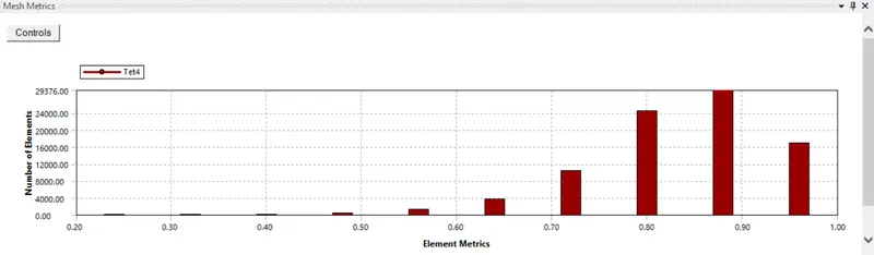
From the above graphs, it is pretty clear that for the different size of meshing, the most of the element qualities were greater than 50%. So, the change in mesh size does not affect the precison of the results that much.

Mesh Independence study:

• Mesh independence or Grid independence study is something we can perform to determine the dependence of the results on the mesh density.
• Comparing the results for various runs for different sizing of the meshing elements . In order to pass, the mesh independence results should be obtained with proper precision.
• Here, we have considered the mesh independence study on short tee below;

Short Tee (Momentum ratio 2)

ELEMENT SIZE (m)	NO OF ELEMENTS	AVERAGE OUTLET TEMPERATURE °C	NUMBER OF ITERATIONS FOR CONVERGENCE	AVERAGE OUTLET VELOCITY MAGNITUDE (m/s)
0.010219(Default)	12568	30.2250°C	140	4.5
0.0050	14378	30.2030°C	137	4.505
0.0025	61426	30.2914°C	128	4.4938

Short Tee (Momentum ratio 4)

ELEMENT SIZE (m)	NO OF ELEMENTS	AVERAGE OUTLET TEMPERATURE °C	NUMBER OF ITERATIONS FOR CONVERGENCE	AVERAGE OUTLET VELOCITY MAGNITUDE (m/s)
0.010219(Default)	12568	27.5500°C	162	6.0139
0.0050	14378	27.5518°C	151	6.0267
0.0025	61426	27.5896°C	145	6.0140

Conclusion:

• Here, we have used the 'K-epsilon' model because we needed a flow simulation turbulent model far from the walls to accurately predict the free stream velocity far from the boundaries rather than the K-omega model which predicts the flow in the viscous sub layers.
• After conducting simulations, as the number of elements increases the computational time also increases.
• By decreasing the element size and making the mesh finer, we can get accurate results and also number of iterations for the convergence takes place will be decreased comparing to the Coarse mesh.
• As we have seen in both the subsections of Case 1, the temperature at the outlet drops down significantly due to high velocity of cold air from the inlet. This is possible due to the turbulent mixing at the tee joint between hot air and cold air because of the high velocity of cold air, which is not possible in the case of low velocity cold air.
• The temperature contour at the outlet for short tee cases shows that some of the high temperature flow sips through without proper mix with the flow. whereas, In the long tee cases, the high temperature air flows and completely mixes with rest of the flow. It is, because of the effectiveness of mixing is low comparing to the long tee's.
• Therefore, we can use the long tee with higher momentum ratio for measuring the effectiveness of mixing in applications due to its low standard deviation in temperature when comparing to the short tee for both momentum ratios.
• For low velocity inlet applications, we can use the short tee for good mixing of fluid's results.