Week 1- Mixing Tee

Aim

Set up a steady state simulation to compare the effectiveness when hot inlet temperature is `36^0C` and cold inlet temperature is `19^0C` using turbulence models `k-epsilon` and `k-omega` for the given two cases.

1. Short mixing tee with a hot inlet velocity of 3 m/s and Momentum ratio of 2, 4.
2. Long mixing tee with a hot inlet velocity of 3 m/s and Momentum ratio of 2, 4.

Objectives

• Compare the effectiveness of `k-epsilon` and `k-omega` turbulence model
• Velocity and temperature contour plots on the cut planes along and across the pipe.
• Velocity and temperature line plots along and across the length of the pipe.
• Perform Mesh independent study for any one case.
• Discuss the effect of length and momentum ratio on results.
• Compare the following values from above cases in a table
  1. Cell count
  2. Average outlet temperature
  3. Number of iterations of convergence

Methodology

In order to perform this steady state analysis, Ansys Fluent from Ansys Workbench has been used. The solver solves the governing equations, which includes momentum, energy equations etc. by the help of some additional equations as per the type of simulation that we are going to perform. Here we are turbulence models `k-epsilon` and `k-omega` for the given two cases. Following steps were carried out as a part of pre-processing.

Step 1: Open Ansys Fluent

Ansys Fluent has been opened from the toolbox window in Ansys workbench.

Step 2: Geometry Creation

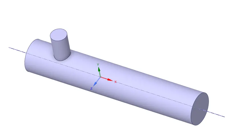
In this step fluid volume is extracted from the mixing tee cad model by the help of extract tool available in SpaceClaim.

Step 3: Naming and meshing of fluid domain

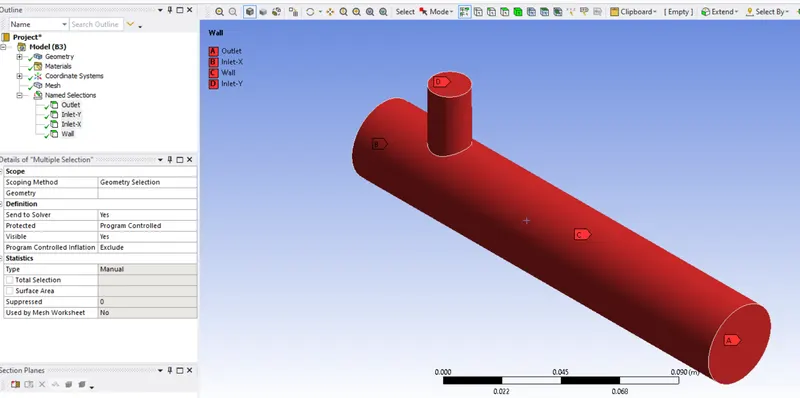
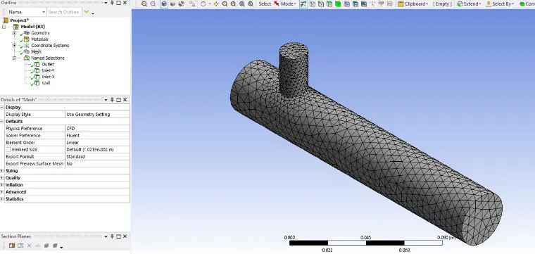
After creating the geometry file the next step is to divide the domain into small parts. Before that we will assign names for different faces to apply boundary conditions easily. After that mesh has been generated by clicking on generate mesh. Here the mesh is generated by default element size.

Step 3: setting up the problem.

Here we setup the problem by applying relevent

• Initial conditions
• Boundary conditions
• Material properties
• Turbulence Models

We will see this step in detail while doing each cases.

Step 4: Post Processing

In this step we analyze the results obtained by the help of contour plots, line plots, charts etc.

SETTING UP THE PROBLEM.

In this section we are going to resolve each objective step by step.

1. Effectiveness of turbulence models of `k-epsilon` and `k-omega`

For this turbulence model study, short mixing tee with a hot inlet velocity of 3m/s and Momentum ratio 2 is used.

The fluid domain and the meshing is done as discussed in the methodology. Here the problem is set up giving initial and boundary conditions for both `k-epsilon` and `k-omega` turbulence model. For this setup module in the Ansys fluent is opened and following changes have been made.

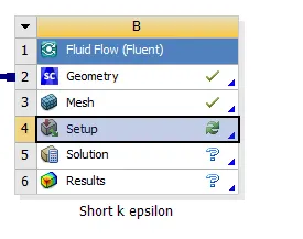
After double clicking the setup, following window is opened. This is where we need to setup the simulation.

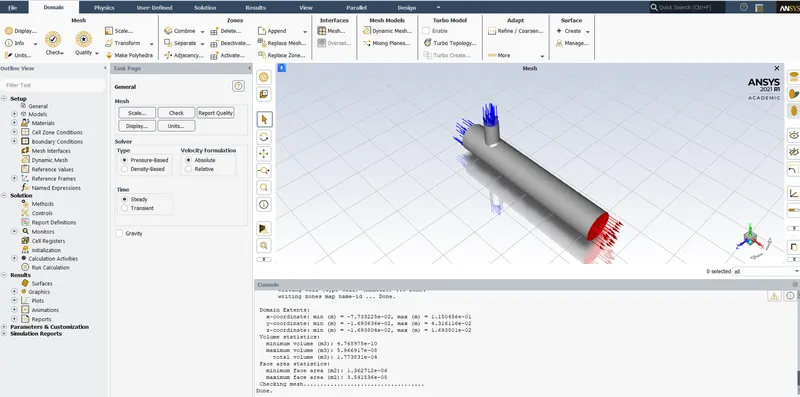
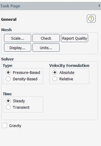
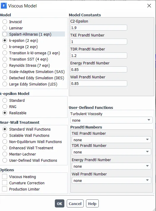
Since the flow is steady state, steady state is selected and since the flow is low velocity means with very less Mach number Pressure based solver is used. Since we are interested in solving the temperature, energy is enabled to use the energy equation. Since the flow can be turbulent we need to incorporate turbulent model by click on viscous menu. From the pop up window K-epsilon realizable model has been picked to perform the simulation with k epsilon `k-epsilon` turbulence model

Next step is to select the material, since air is our working fluid we are not changing anything.

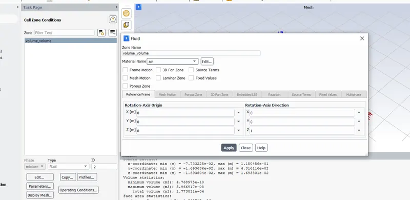
After this we will update working fluid in cell zone condition as air (by default it is air).

This can be accessed under Physics->Zones->cell zones

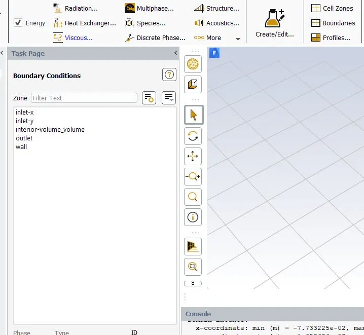
Next step is to assign the Boundary condition. Our boundary conditions are,

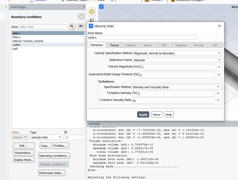
Inlet-X (Hot air); type – Velocity inlet 3 m/s Momentum ratio = Cold air velocity/hot air

Temperature 2 = cold air velocity /3

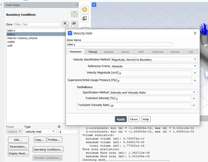
Cold air velocity = 6 m/s

Inlet-Y (Cold air); type – Velocity inlet 6m/s

Temperature

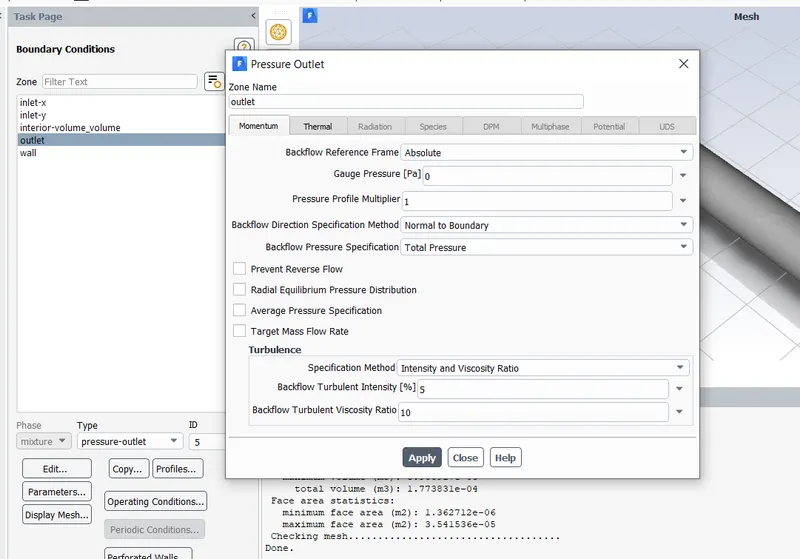
Outlet; type – Pressure outlet

Gauge pressure = 0

These changes have been made in the boundary conditions that can be accessed under

Physics->Zones->Boundaries

The above boundary conditions have been updated at appropriate boundaries.

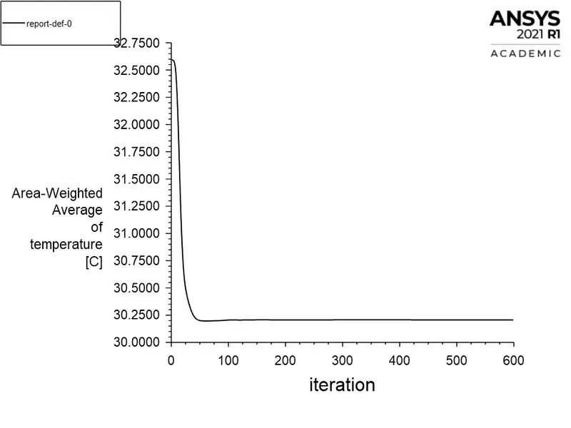
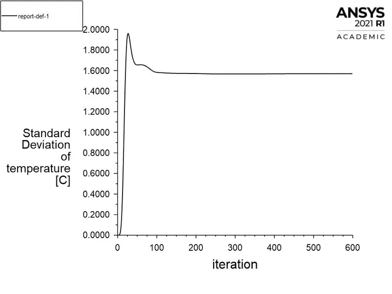
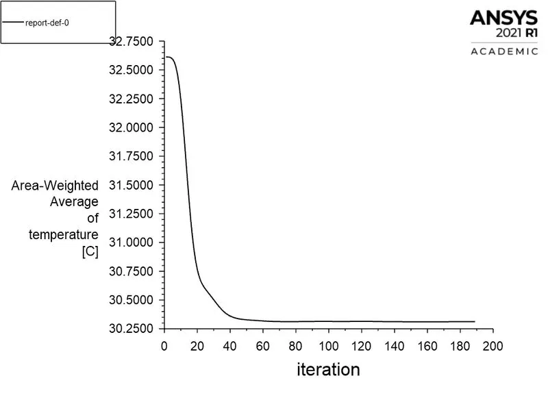
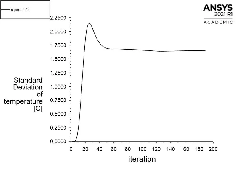
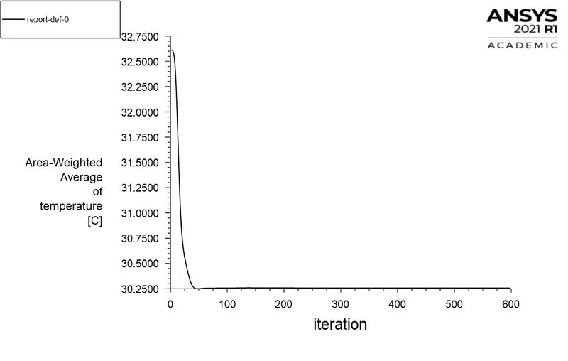
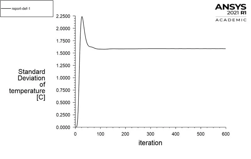
As of now the setup has been completed. As the simulation progresses, we will monitor the area weighted average of temperature at the outlet. Since it is a mixing problem, to understand the effectiveness of mixing we will take the standard deviation of temperature at the outlet.

Now it is time to initialize the solution. In CFD analysis the solver is solving for pressure, velocity and other variables. Since we have provided only velocity at the inlets the solver need to get starting points for all these variables. For this purpose, initialization is used. Here hybrid initialization is used to initialize the solution.

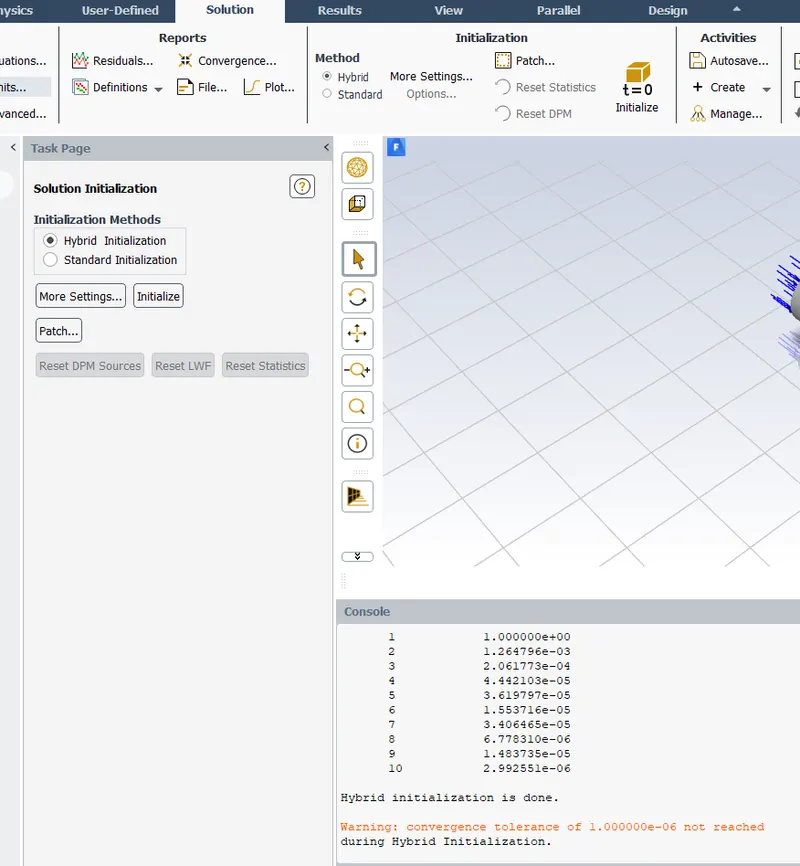
After initialization, click on run after giving iteration number as 600.

The same process is repeated to get solution using k-omega SST model. For this k omega from the viscous model is selected and ran the simulation by providing number of iterations.

Post Processing.

After running the above setup, following results were obtained.

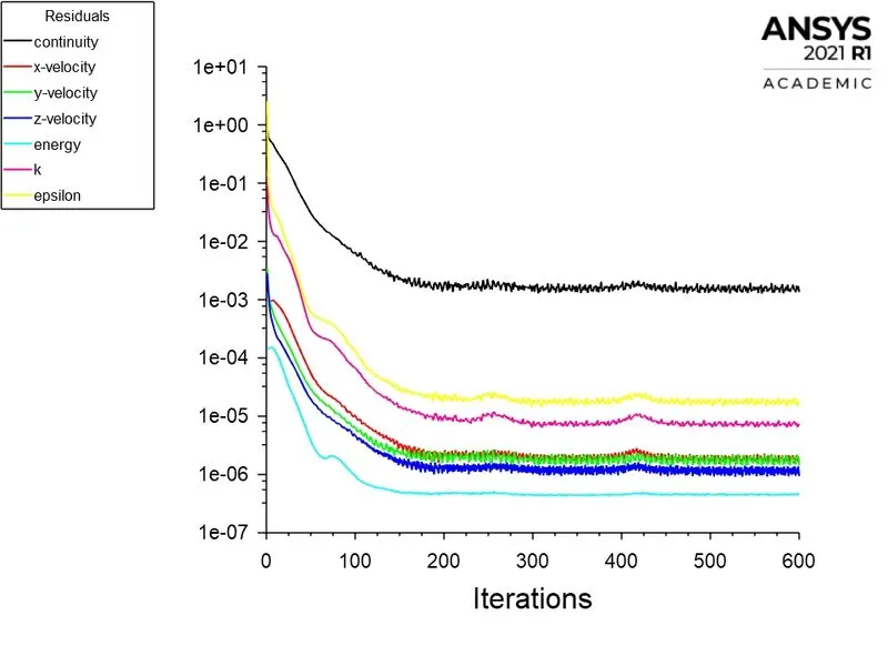
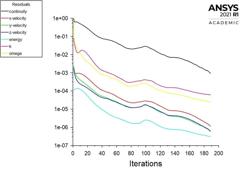
• Convergence plots

1). Using K-Epsilon

2). Using K-Omega SST

• Temperature and velocity Contours

1). Using K-Epsilon

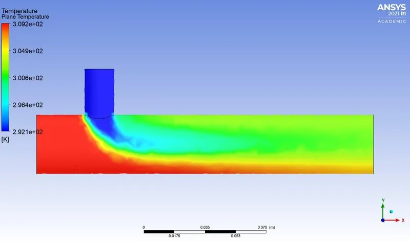
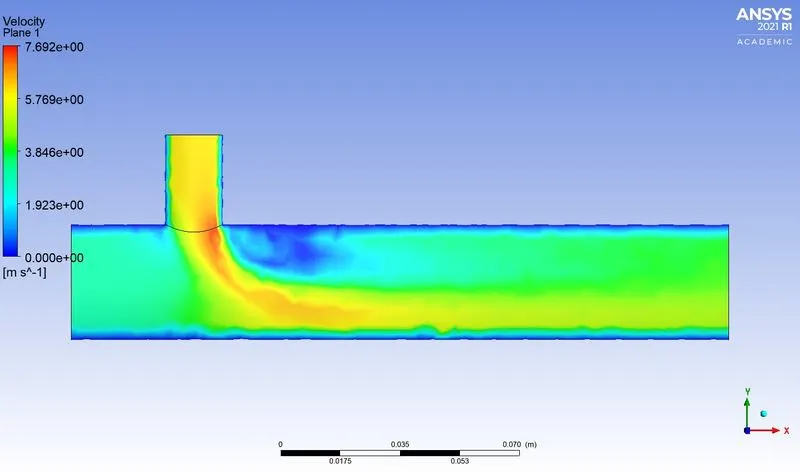
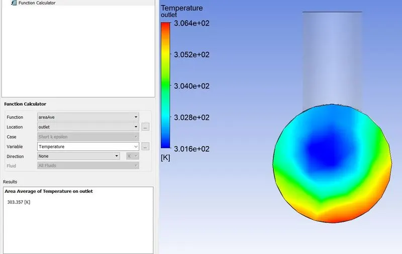
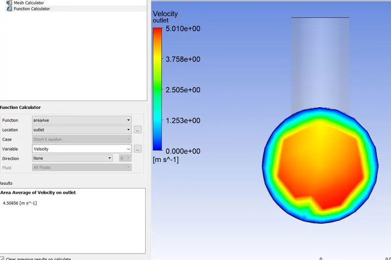
Average Temp at outlet = 303.38K ; Average Velocity at outlet = 4.508 m/s

2). Using K-Omega SST

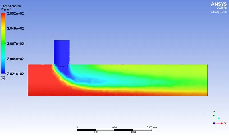
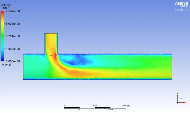
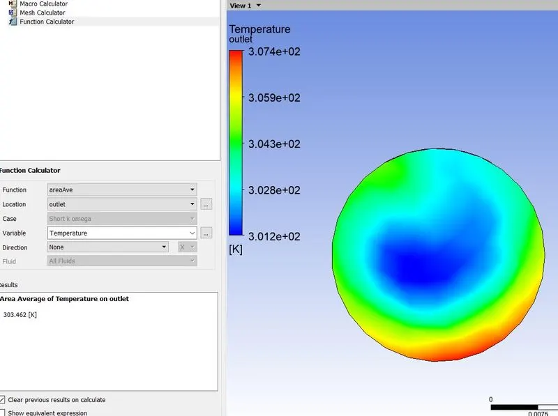
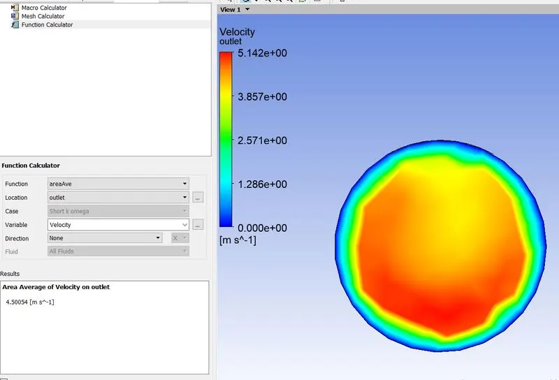
Average Temp at outlet = 303.38K ; Average Velocity at outlet = 4.5 m/s

• From the convergence plot, it is clear that for the same problem setup, K-omega model needed only 189 iterations to converge to the solution. So we can say that k-omega model is faster than the K-epsilon viscous model.
• Also for both the models the solutions are almost same with very minute error.
• In general, K-omega model is very efficient in capturing the flow phenomena’s in the vicinity of boundaries and k-epsilon model is very efficient in capturing flow phenomena’s away from the boundaries. Since we are dealing with mixing tee problem we will be using k-epsilon model for the coming simulations

2. Study on mixing Tee length with momentum ratios 2 and 4

Case 1: Short mixing tee

Momentum Ratio = 2

The following changes were made in the boundary condition

Inlet-X (Hot air); type – Velocity inlet 3 m/s Momentum ratio = Cold air velocity/hot air

Temperature = `36^0C` 2 = cold air Velocity/3

Cold air Velocity= 6 m/s

Inlet-Y (Cold air); type – Velocity inlet 6m/s

Temperature = `19^0C`

Post Processing

• Convergence plots

• Temperature and Velocity contours

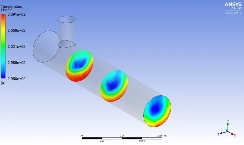
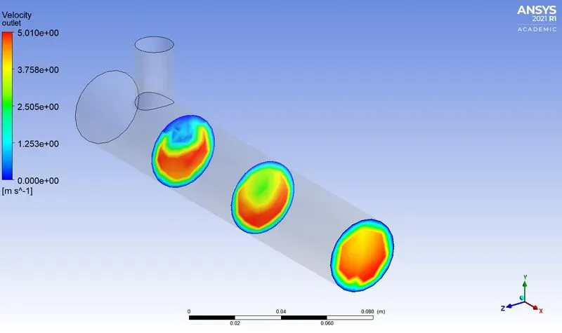
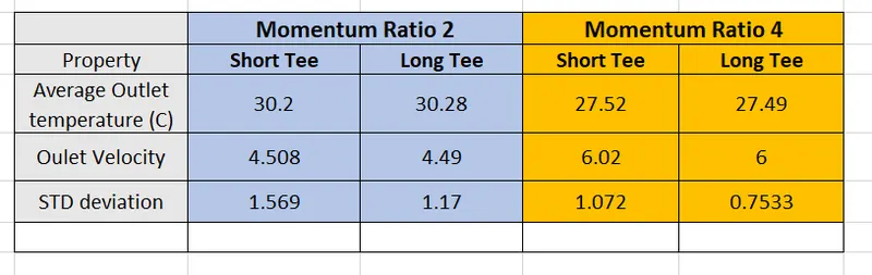
Average Temperature at outlet = `30.2^0C`

Average velocity at outlet = 4.508 m/s

Standard deviation of Temp at outlet = 1.569

Momentum Ratio = 4

The following changes were made in the boundary condition

Inlet-X (Hot air); type – Velocity inlet 3 m/s Momentum ratio = Cold air velocity/hot air

Temperature `36^0C` 4 = cold air/3

Cold air = 12 m/s

Inlet-Y (Cold air); type – Velocity inlet 12 m/s

Temperature `19^0C`

Post Processing

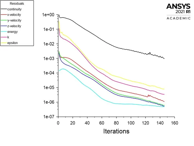
• Convergence plots

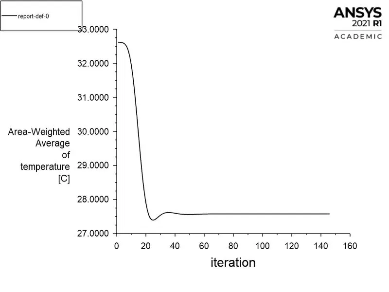
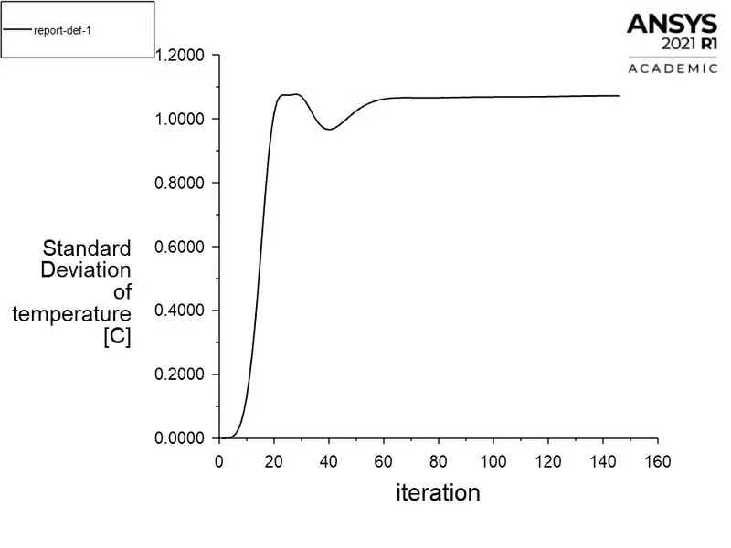
• Temperature and Velocity contours

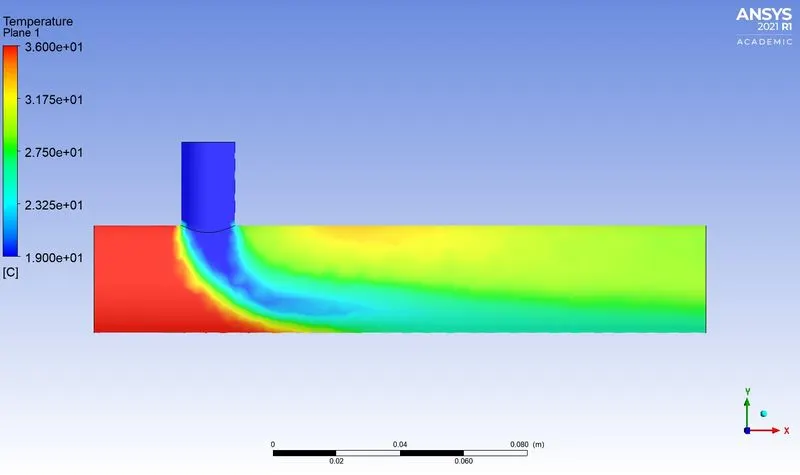
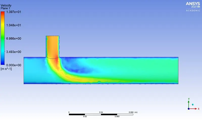
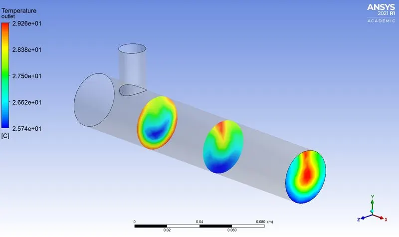
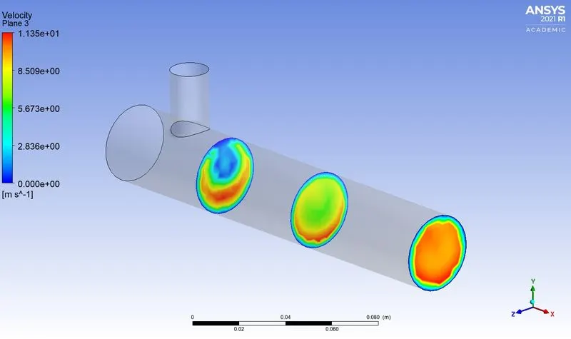
Average Temperature at outlet =

Average velocity at outlet =

Standard deviation of Temp at outlet = 1.072

B). Case 2 : Long mixing tee

1). Momentum Ratio = 2

The following changes were made in the boundary condition

Inlet-X (Hot air); type – Velocity inlet 3 m/s Momentum ratio = Cold air velocity/hot air

Temperature = `36^0C` 2 = cold air Velocity/3

Cold air Velocity= 6 m/s

Inlet-Y (Cold air); type – Velocity inlet 6m/s

Temperature = `19^0C`

Post Processing

• Convergence plots

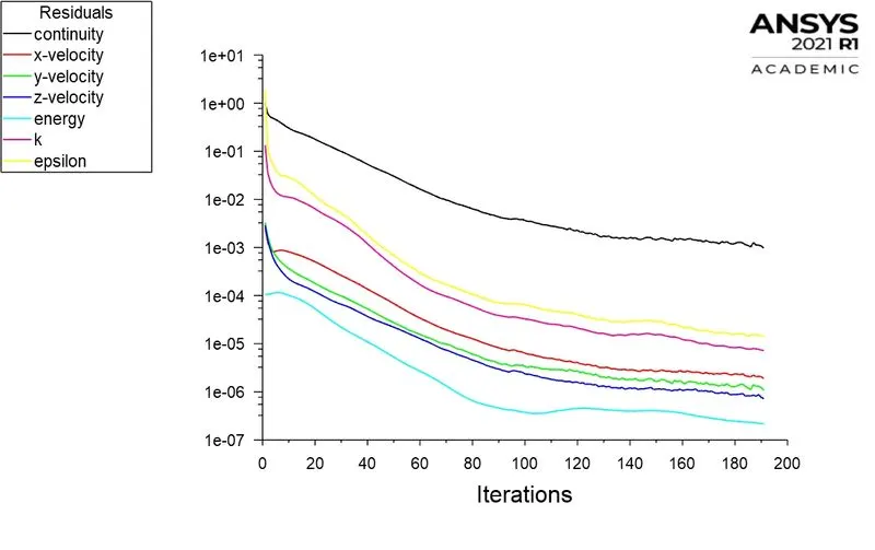
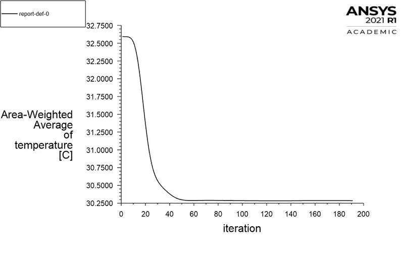
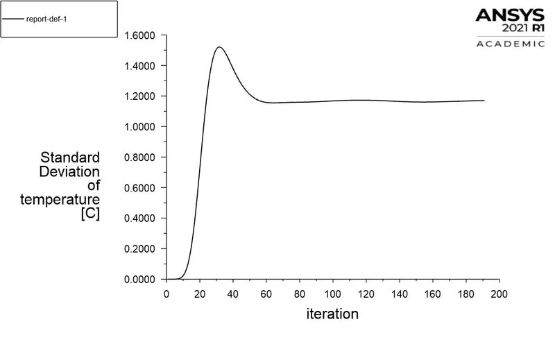
• Temperature and Velocity contours

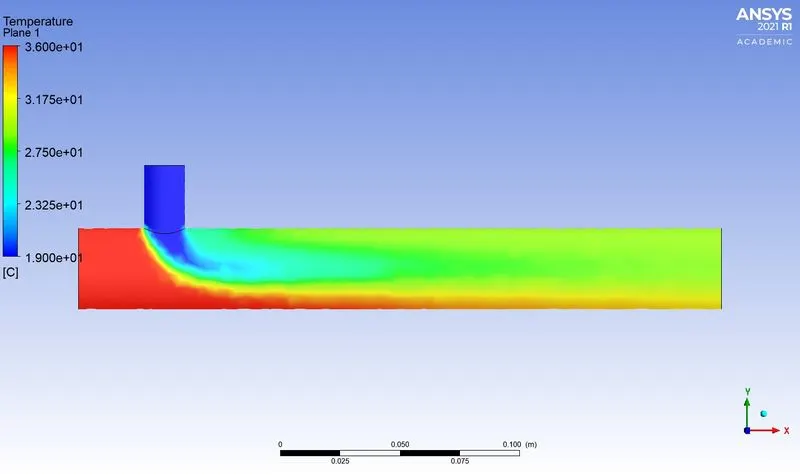
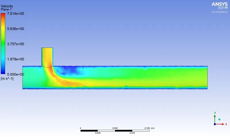
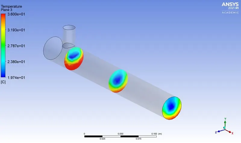
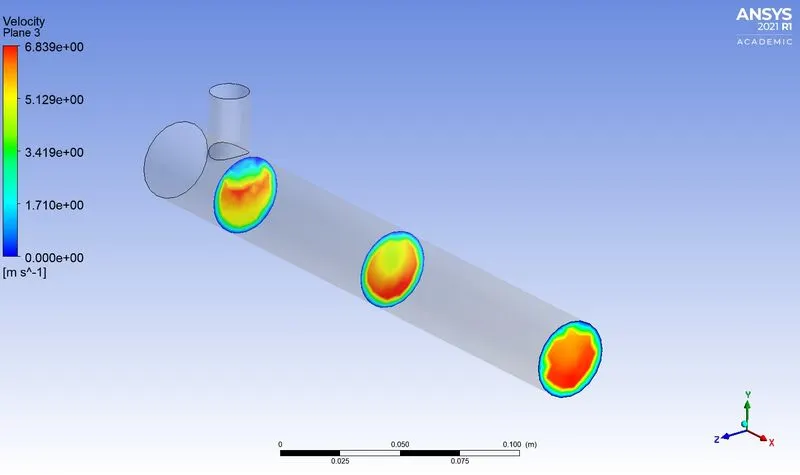
Average Temperature at outlet = `30.28^0C`

Average velocity at outlet = 4.49 m/s

Standard deviation of Temp at outlet = 1.17

2). Momentum Ratio = 4

The following changes were made in the boundary condition

Inlet-X (Hot air); type – Velocity inlet 3 m/s Momentum ratio = Cold air velocity/hot air

Temperature = `36^0C` 4 = cold air Velocity/3

Cold air Velocity= 12 m/s

Inlet-Y (Cold air); type – Velocity inlet 12 m/s

Temperature = `19^0C`

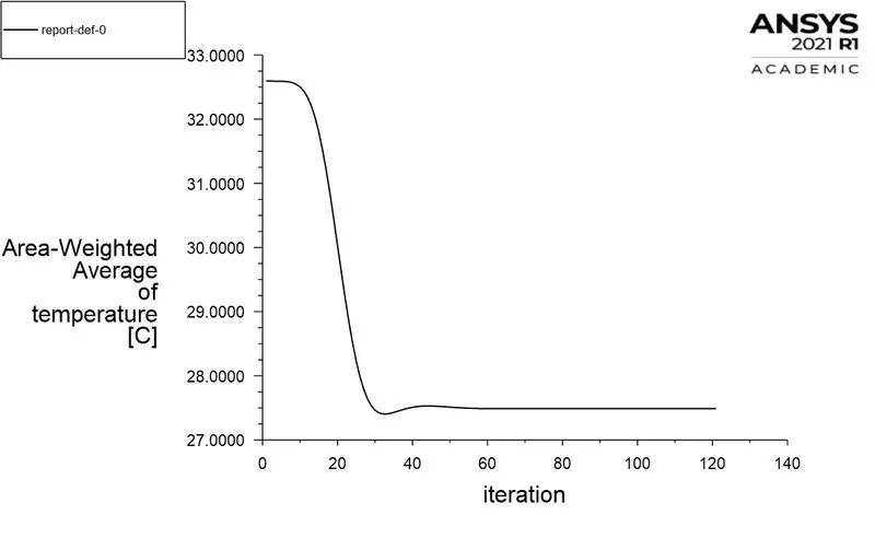
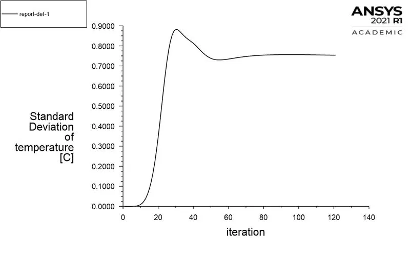
Post Processing

• Convergence plots

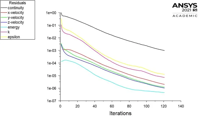
• Temperature and Velocity contours

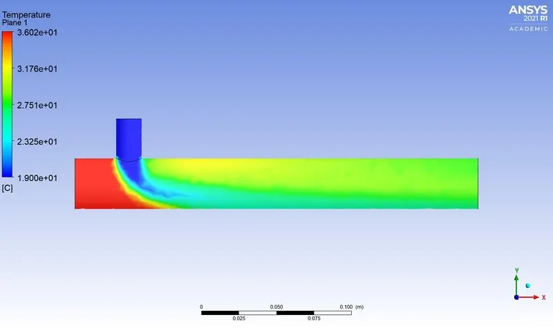
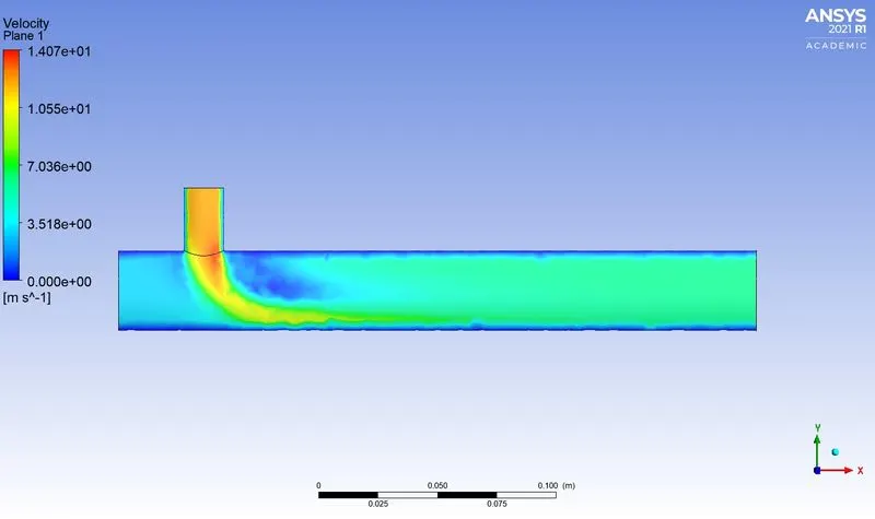
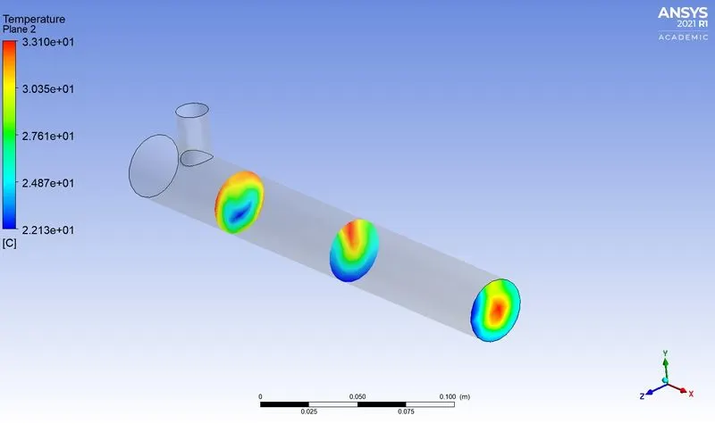
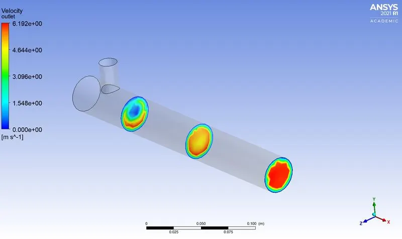
Average Temperature at outlet = `27.49^0C`

Average velocity at outlet = 6.00 m/s

Standard deviation of Temp at outlet = 0.7533

• From the above simulations it is clear that as the length of the tee increases we are getting a better standard deviation in temperature, which means that the hot and cold air is mixing each other in a better manner than in short tee. Also we can observe Temperature and velocity are almost same for both short and long mixing tee at a given momentum ratio. The following table shows the segregated results.

3. Study on Grid independency

In order to study the grid independency, a short mixing tee with momentum ratio 2 has been used. The grid size can be changed in in mesh properties while preprocessing. The following 3 different grid sizes have been used to validate the study.

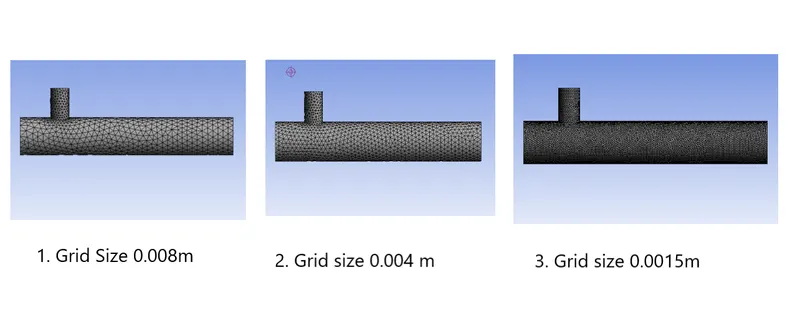
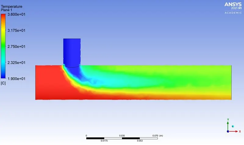
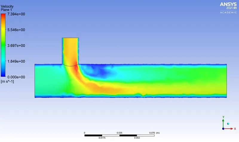
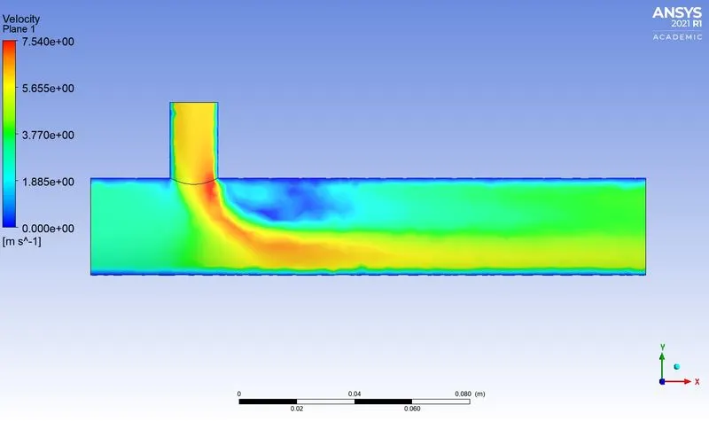
After running simulation for each grid size shown as above, temperature and velocity contours obtained as follows. Also a detailed tabular data has been provided for a better understanding.

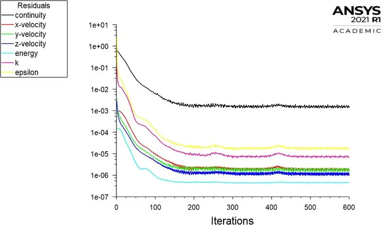
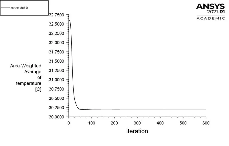
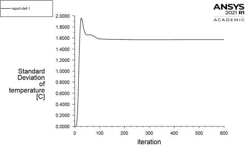
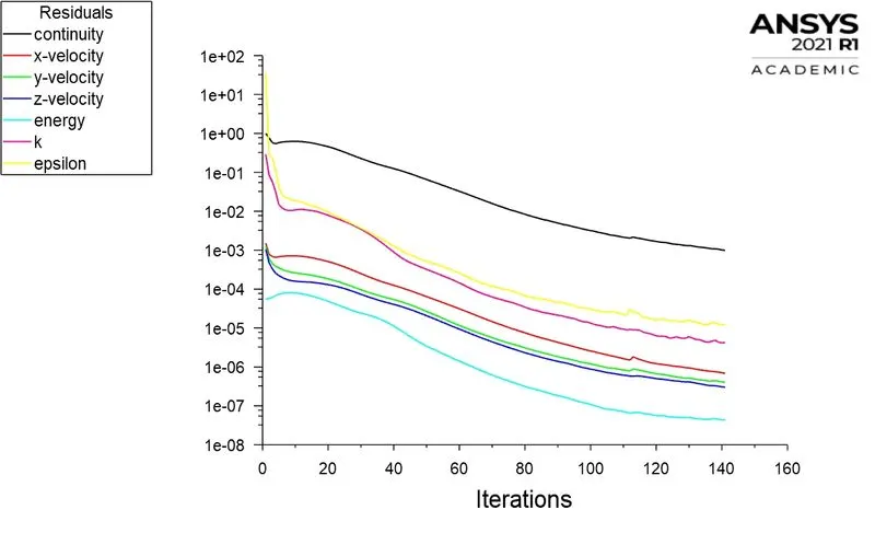
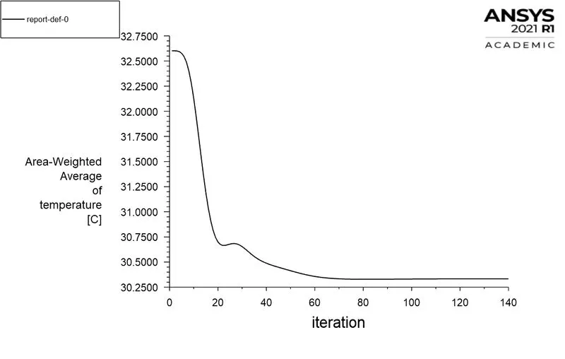
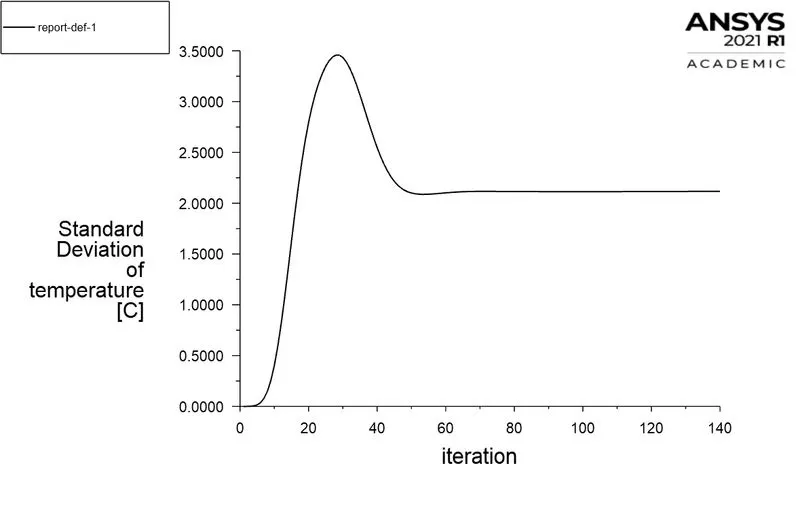
• Convergence Plot

1). Grid size 0.008 m

2). Grid size 0.004 m

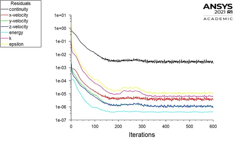
3). Grid size 0.0015 m

• Temperature and velocity Contour

1). Grid size 0.008 m

Grid size 0.004m

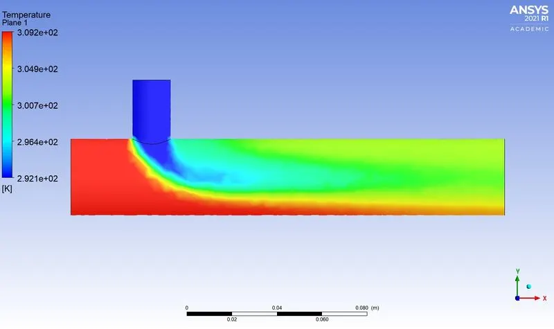
3).Grid size 0.0015 m

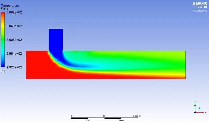
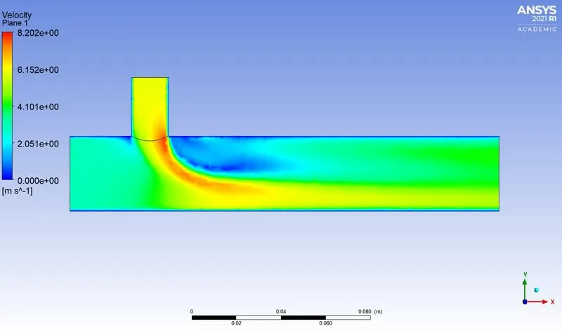
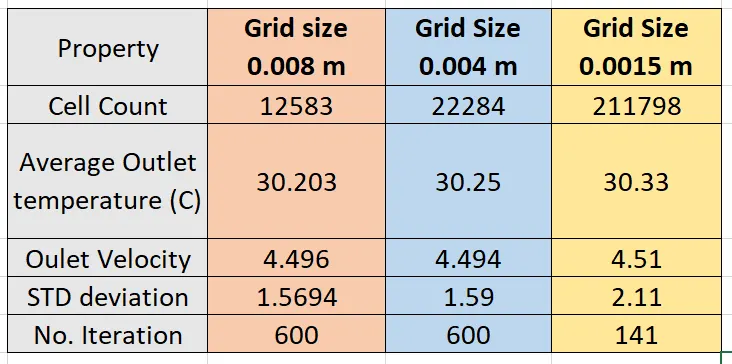
• From the above study, we can observe that the average outlet temperature and velocity does not change depending upon the size of the grid. Hence we can easily prove the grid independency here. The above table can be used to confirm this easily.
• Another thing to notice is that, as the number of cells increases the computation time also increases heavily. Even though, the temperature as well as velocity contours getting much more refined as the number of cells increases. We can observe from the plots that refined mesh gives a detailed mixing region. (grid size 0.0015 m)

CONCLUSIONS

The above studies on the simulation of mixing tee, following conclusions are made,

• In CFD, viscous model k epsilon is used to study the flow phenomenon away from the boundaries and k omega is used to study the flow phenomenon near the boundaries. K omega mode is giving converged solution than k epsilon model.
• As the length of the tee increases the mixing efficiency is inceasing. Also as the momentum ratio increases the mixing efficiency is increasing.
• For a given length of mixing tee, increasing the momentum ration will provide a good mixing efficiency.
• Another conclusion is that, the final results are independent on the size of the grid. However, smaller the grid size larger the resolution of results but it also consumes time.