Week 1: Channel flow simulation using CONVERGE CFD
Channel flow simulation using CONVERGE CFD
Aim:
Simulating the flow through a channel using CONVERGE CFD.
Objectives:
- Able to simulate the channel flow for three different base mesh sizes
- different base mesh sizes are,
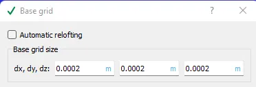
- dx = 2e-4m, dy = 2e-4m, dz = 2e-4m
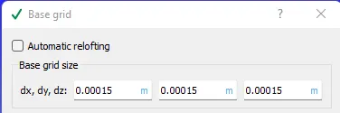
- dx = 1.5e-4m, dy = 1.5e-4m, dz = 1.5e-4m
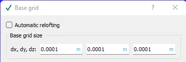
- dx = 1.0e-4m, dy = 1.0e-4m, dz = 1.0e-4m
- different base mesh sizes are,
- Explain Results & plots for velocity, pressure, mass flow rate, and total cell count for all 3 base mesh sizes.
Flow simulation in CONVERGE done in 3 steps:
- Geometry preparation and Case setup :
- We use Converge GUI(Graphical User Interface) to set up the case and export input files.
- Solving the problem using input files:
- These input files are solved by Converge in the Terminal (Command-line interface). We USed Cygwin for the command line terminal.
- Post-processing results:
- We convert our solution into Paraview binary format to post-process the results in Paraview
Geometry preparation in CONVERGE CFD:
- Geometry preparation:
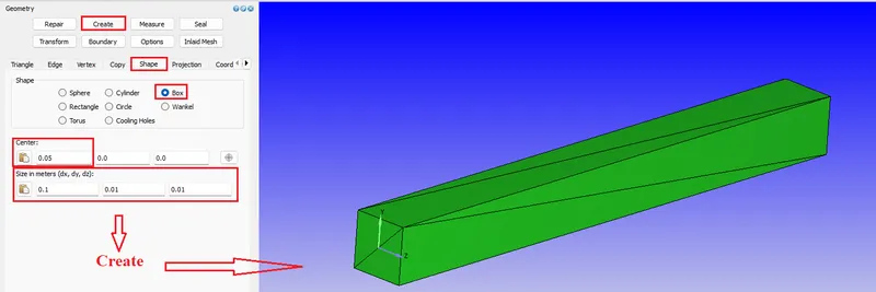
- Under the Geometry section, Create a rectangle channel for the flow domain.
- Under the Geometry section, Create a rectangle channel for the flow domain.
- Boundary setting:
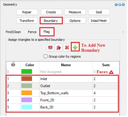
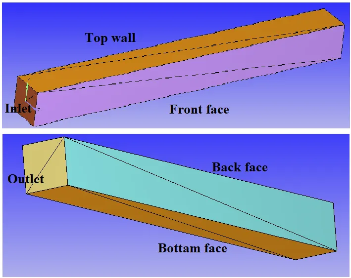
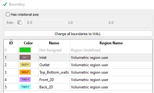
- We have to set Inlet, Outlet, Top and Bottom walls, Front & Backface boundaries for the above-created geometry.
- By default In CONVERGE, all the surfaces are made up of triangles we have to select respective triangle faces for the boundary.
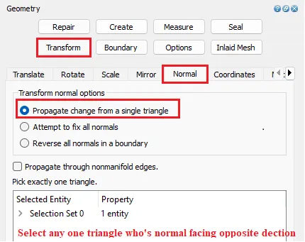
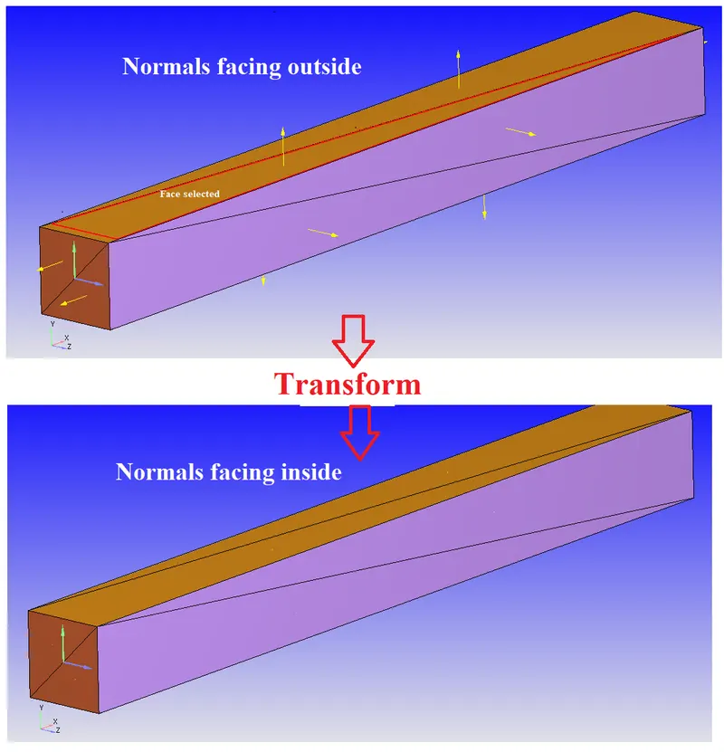
- Normal Transformation:
- All the face normals directions should be towards the flow region.
- In this fluid is flowing through the channel but normals are facing outwards. We have to transform the normal's direction.
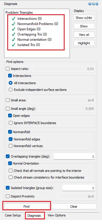
- Diagnosis:
- Checking for any interactions, open edges, etc.
Case Setup in CONVERGE CFD:
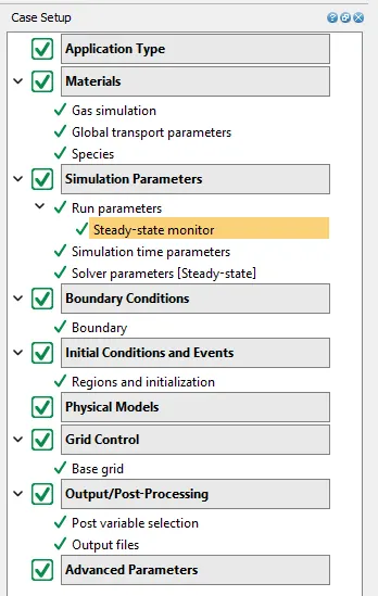
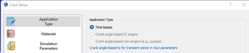
- Application Type :
- Materials:
- Set default values in Gas Simulation & Global transport parameters.
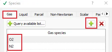
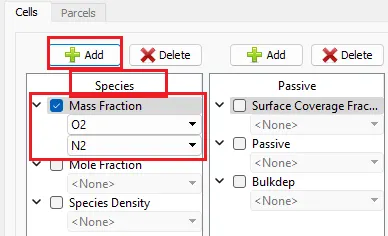
- Species: Add Gas species O2 & N2.
- Initial Conditions and Events:
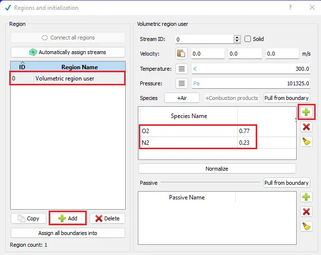
- Add Volumetric region in regions
- Add species by modifying their concentrations so that we can clearly observe the difference in post-processing.
- Boundary conditions:
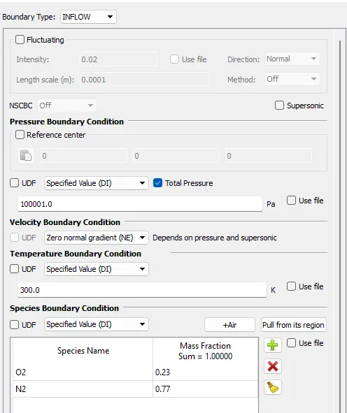
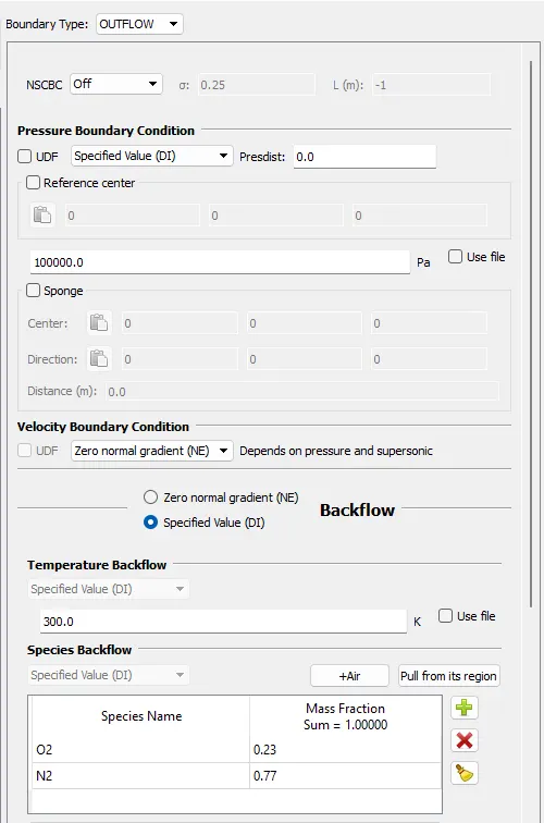
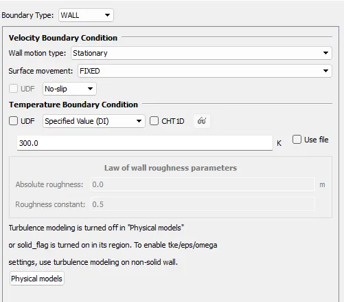
- Defining boundary type and conditions:
-
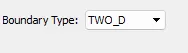
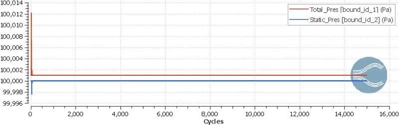
Boundary Name Type Boundary Condition Value Species Inlet INFLOW Total Pressure 100001 Pa O2 : 0.23 & N2 : 0.77 Outlet OUTFLOW Pressure 100000 Pa O2 : 0.23 & N2 : 0.77 Top_Bottom_walls WALL No-Slip Front_2D TWO_D Back_2D TWO_D - INLET:
- OUTLET:
- Top_Bottom_walls
- FRONT_2D & BACK_2D
- INLET:
- Defining boundary type and conditions:
- Simulation Parameters:
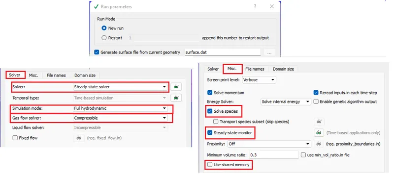
- Run Parameters:
- Selecting the Solver & solver type. informing additional things to solve (Energy & Momentum equations) and monitoring steady-state.
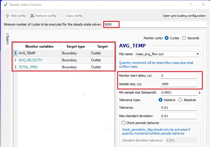
- Steady-state monitor:
- In this, we have to Add monitor variables to be monitored during the simulation at different boundaries.
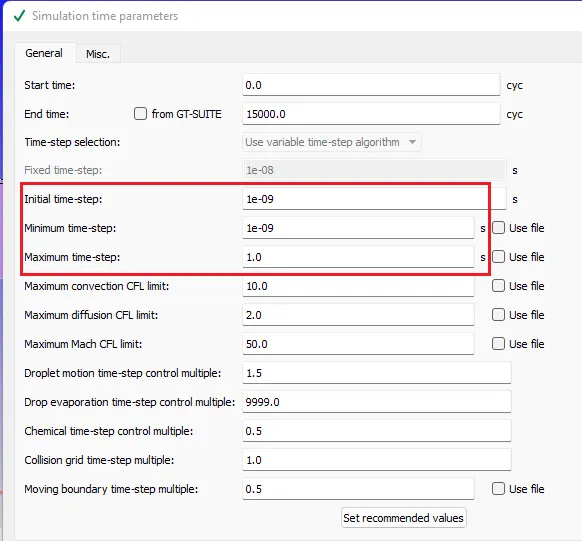
- Simulation Parameter:
- defining initial, Minimum & Maximum Time step sizes.
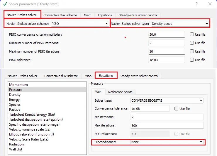
- Solver Parameters:
- Solver Scheme to PISO and Density-based solver.
- under Equations window set precondition to None for all the variables.
- Run Parameters:
- Physical Models:
- Uncheck the Turbulence
- Grid Control:
- This is the section where we define meshing size(Grid size).
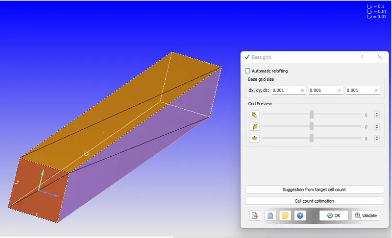
- dx = 2e-4m, dy = 2e-4m, dz = 2e-4m
- dx = 1.5e-4m, dy = 1.5e-4m, dz = 1.5e-4m
- dx = 1.0e-4m, dy = 1.0e-4m, dz = 1.0e-4m
- dx = 2e-4m, dy = 2e-4m, dz = 2e-4m
- This is the section where we define meshing size(Grid size).
- Output/Post-Processing
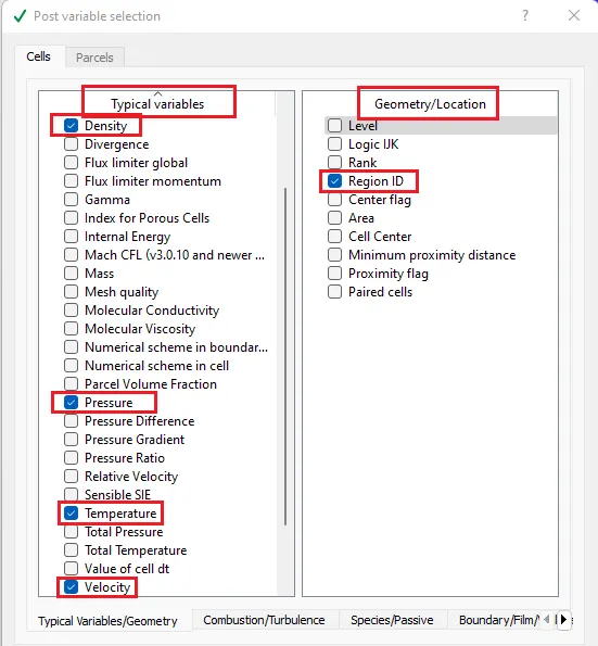
- Post Variable selection: select the variables to be monitored for post-processing.
- Post Variable selection: select the variables to be monitored for post-processing.
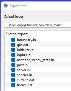
- Exporting Input files:
- Export the input files
- Export the input files
Solving Channel Flow in Cygwin:
- Go to the directory where input files are exported
- Make mpiexec.exe & converge.exe files globally available.
- "mpiexec.exe -n 4 converge.exe restricted </dev/null> logfile &"
- Use above mentioned line to start calculation in the background
- mpiexec.exe & converge.exe are executable applications to solve the problem
- -n 4:- number of processors
- restricted:- my license is a restricted one.
- </dev/null> logfile:- creates temporary memory to save data with name as logfile at a particular iteration
- & :- To run Calculation in Background
- "tail -10 logfile" command is used to view the last 10 lines of the logfile.
- "mpiexec.exe -n 1 post_convert_30_serial_64" command used to convert output files to paraview binary format, so that they can be processed in the paraview.
Post Processing and Results from Paraview:-
open "..vtm" group file in paraview. This group contains all the solution files.
- Case 1: dx = 2e-4m, dy = 2e-4m, dz = 2e-4m
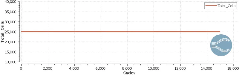
- Total cells = 25000
- Simulation time
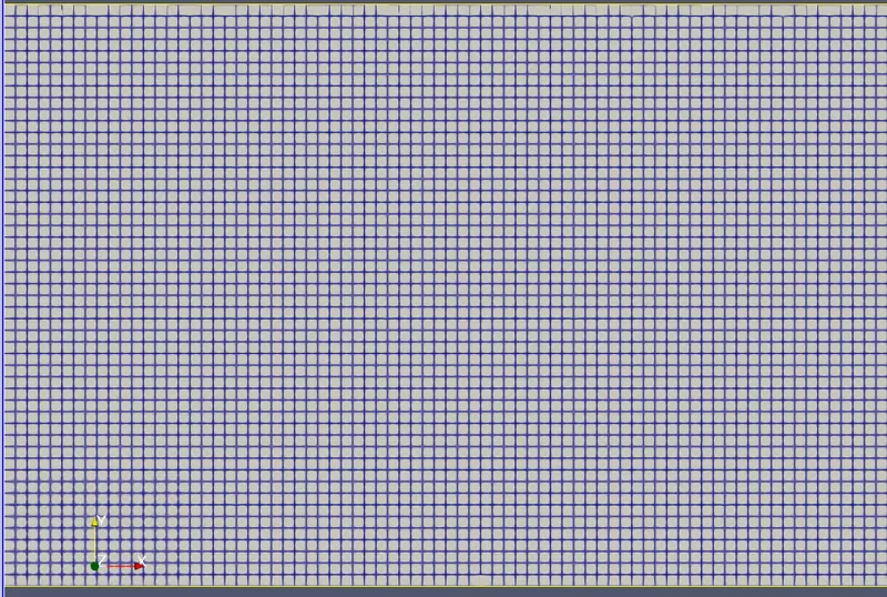
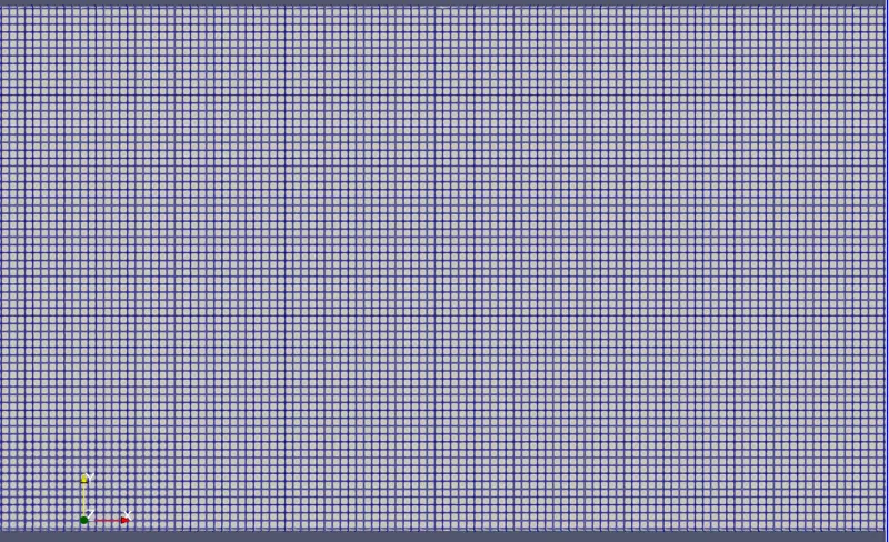
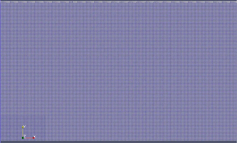
- Mesh
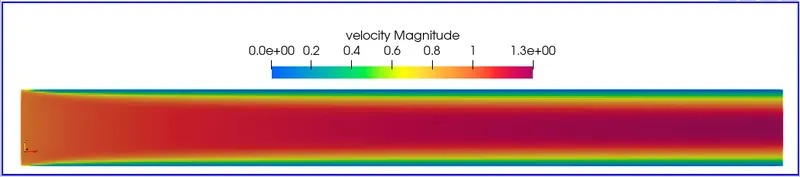
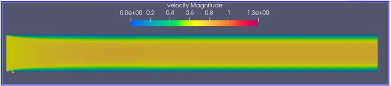
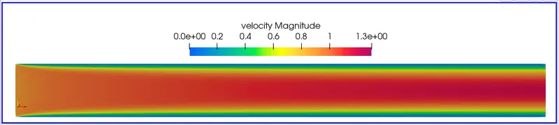
- Velocity Contour
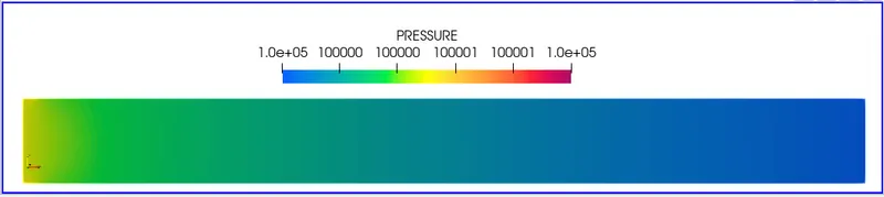
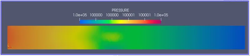
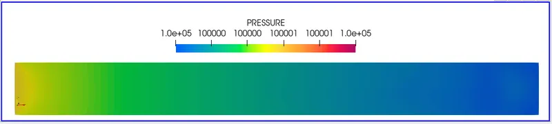
- Pressure Contour
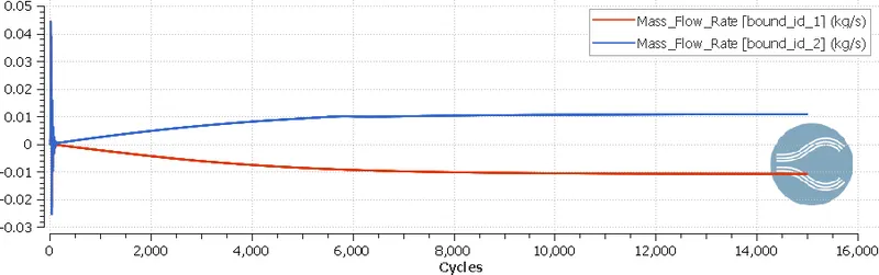
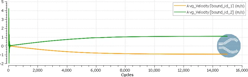
- Plots:
- bound_id_1 = inlet
- bound_id_2 = outlet
- Case 2: dx = 1.5e-4m, dy = 1.5e-4m, dz = 1.5e-4m
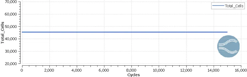
- Total cells = 45420
- Simulation time
- Mesh
- Velocity Contour
- Pressure Contour
- Plots
- bound_id_1 = inlet
- bound_id_2 = outlet
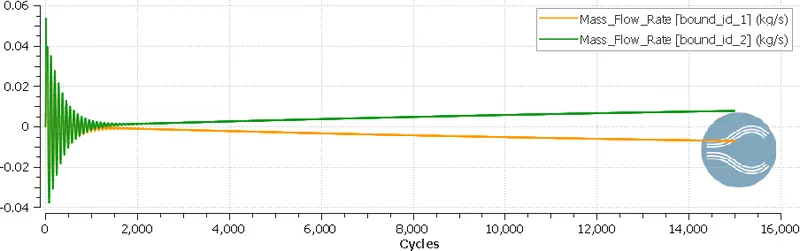
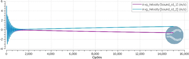
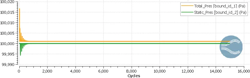
- Case 3: dx = 1.0e-4m, dy = 1.0e-4m, dz = 1.0e-4m
- Total cells = 100000
- Simulation time
- Mesh
- Velocity Contour
- Pressure Contour
- Plots
- bound_id_1 = inlet
- bound_id_2 = outlet
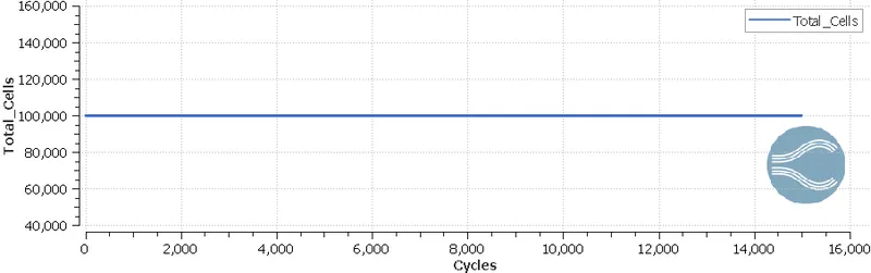
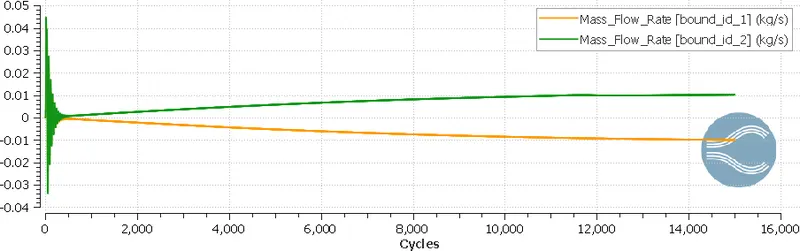
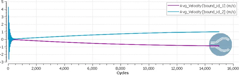
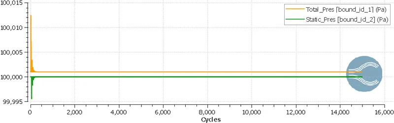






Conclusion:
- As the number of cell count increases solution accuracy and simulation time increase.