Week 1: Channel flow simulation using CONVERGE CFD
Aim
- To setup a steady state channel flow
- Run the simulation for 3 different cases of mesh sizes
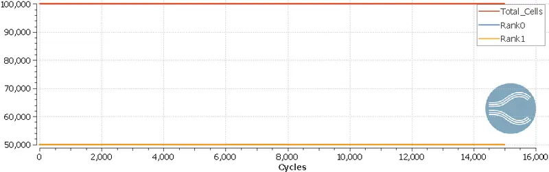
- Obtain plots for velocity, pressure,mass flow rate and total cell count for all 3 base mesh sizes.
- Upload an animation to youtube and attach the link here using the add media option. Explain the development of the flow using the animation
Objective
- Create the geometry
- Setting up the flow case
- Export input files to a folder
- Copy converge.exe and mpiexec.exe to the folder
- Run the simulation using CYGWIN
- Using converge post convert the obtained 3D files to a readable file type for paraview (Ensight or VTK file)
- Open the converted files through paraview and post process the results
Setup
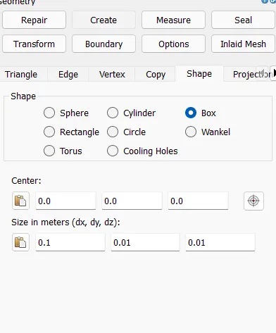
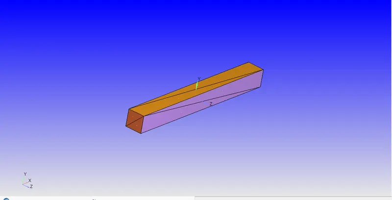
- Geometry is created from the create option availible in the user interface
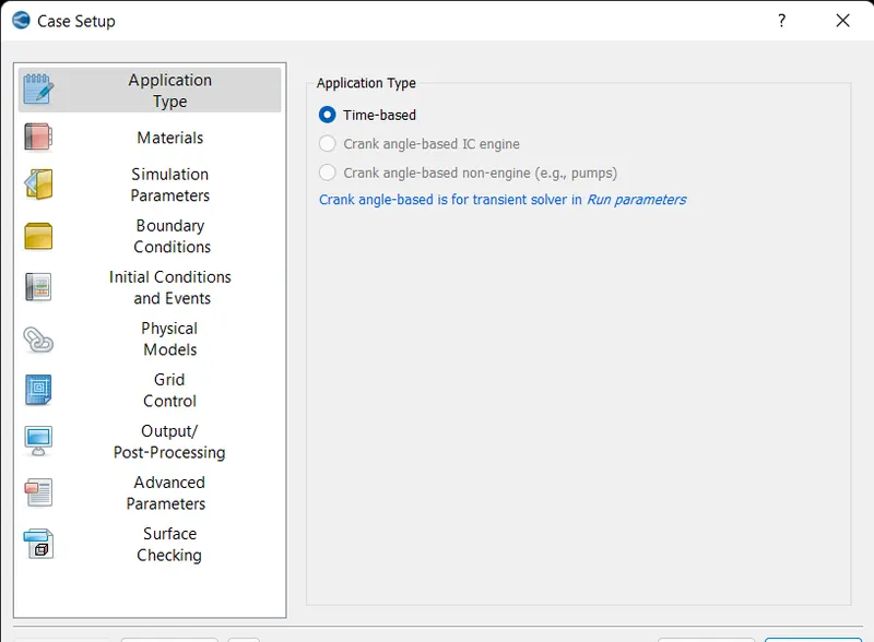
- Case set up is set to time based
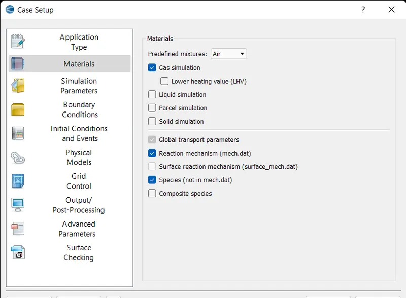
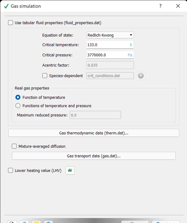
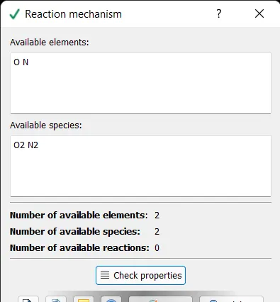
- Material is set to air which contains 77% of nitrogen and 23% oxygen
- A gas simulation was enabled
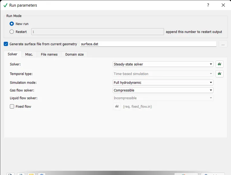
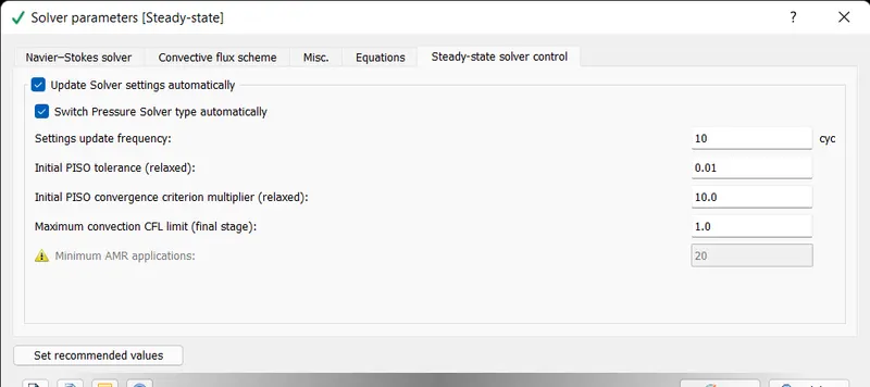
- Steady state analysis is enabled in Simulation run parametres
- In simulation parametres steady state monitor was enabled
- The minimuim number of cycles to be executed is set to 5000
- In simulation time parametres the end time is set to 15000 cycles with initial and minimum time step is set to 1e-9 and maximum time step is set to 1,The convection CFL limit is set to 1
- In solver parametres the navier stokes scheme is set to PISO also the CFL limit for convection is changed to the same value as 1,A pressure based calculation is enabled
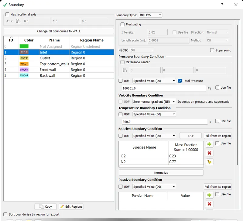
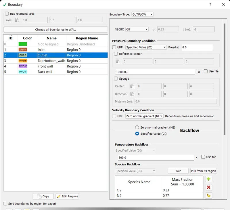
- For boundary conditions the inlet pressure is set to one pascal above 1 bar and for the outlet it is set to 1 bar
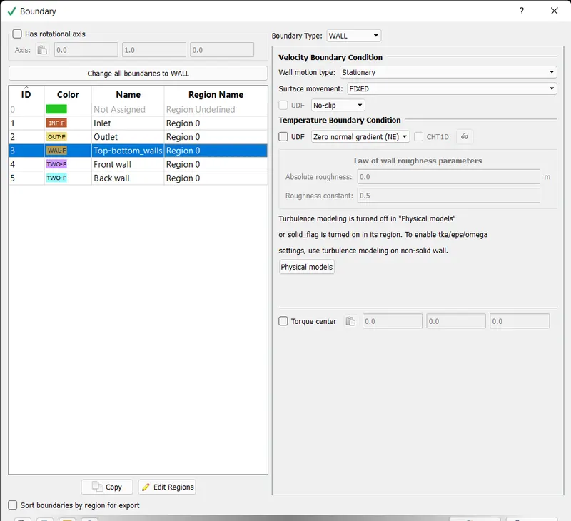
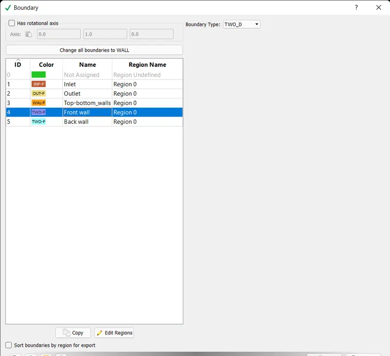
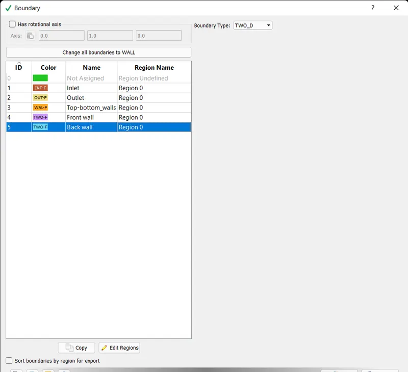
- Inlet boundary type is set to Inflow whereas the outlet is set to outflow,the bottom_top_walls boundary type set to no slip walls and the othe two face is set to TWO-D
- Also at the inlet and outlet the presence of air was also given
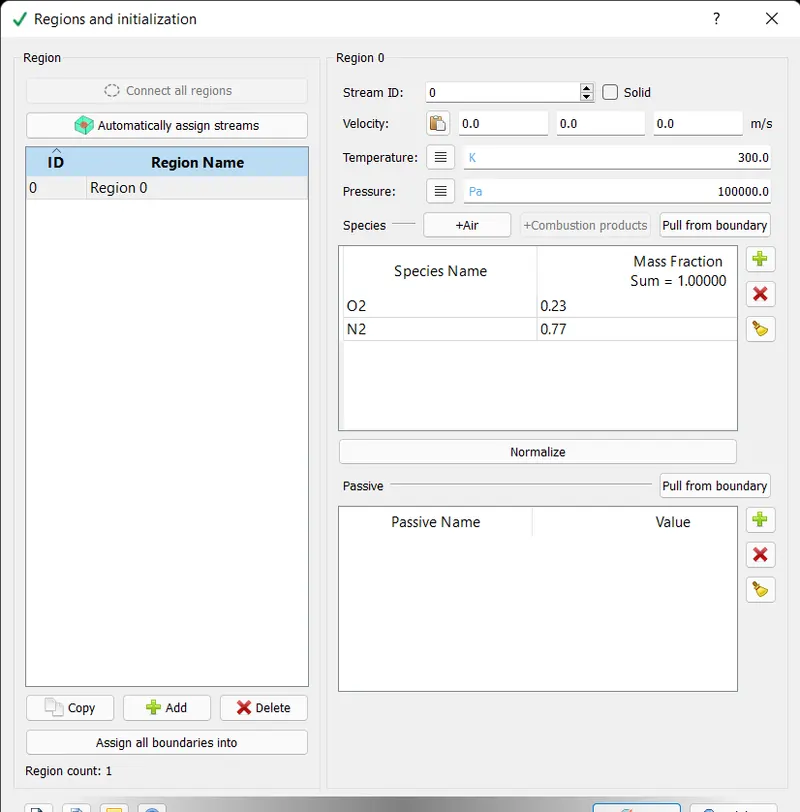
- In the region and initialisation , the initial pressure was set to 1 bar and a region was created containing air as fluid
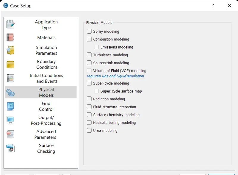
- Turbulance model was disabled in the physical models
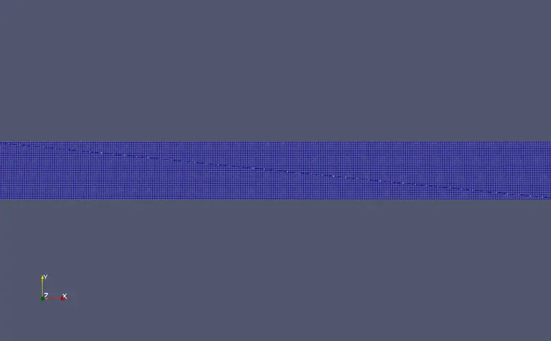
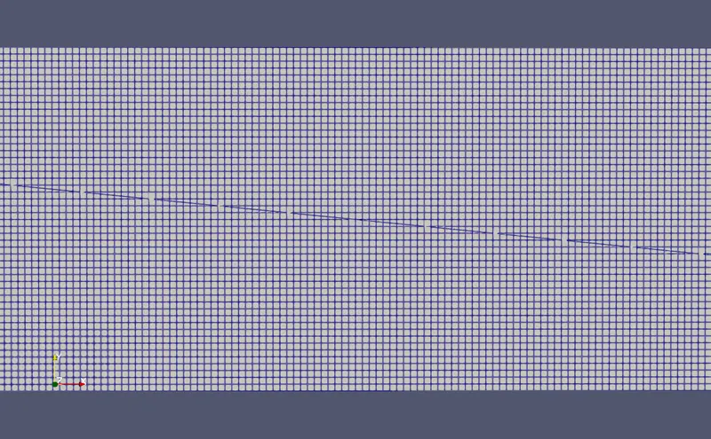
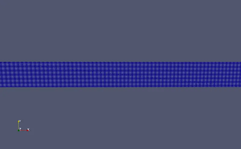
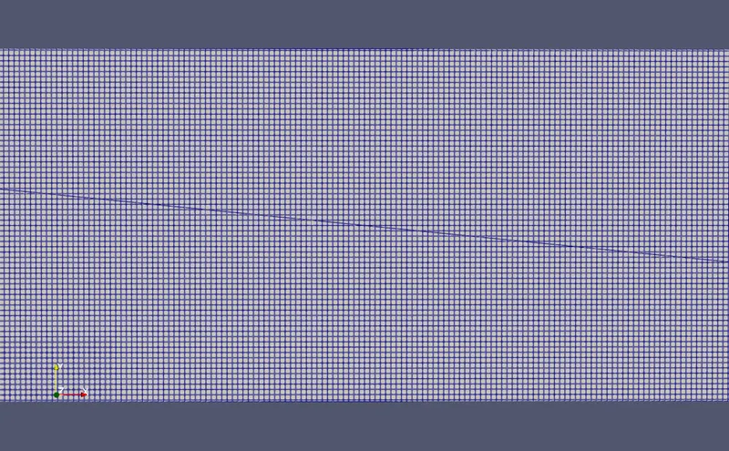
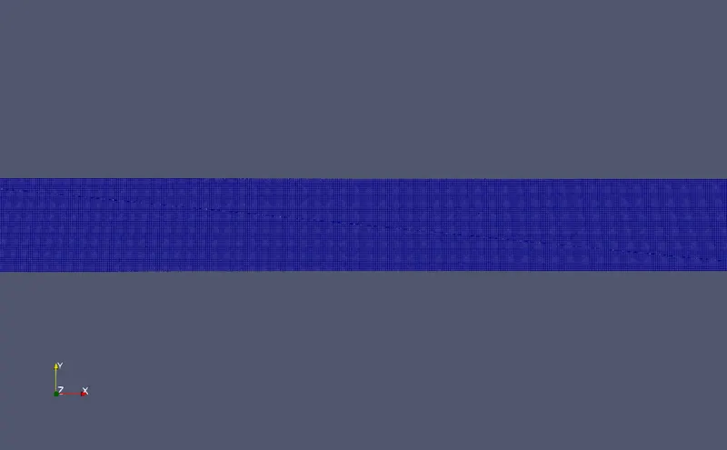
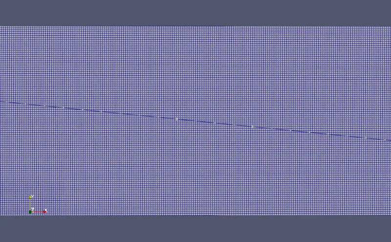
- In the grid control I have given different values for each cases, For case 1 , the mesh size is set to 2e-4m for dx,dy and dz,For case 2 the mesh size was set to 1.5e-4m and for Case 3 the ,esh size in every direction was 1e-4m
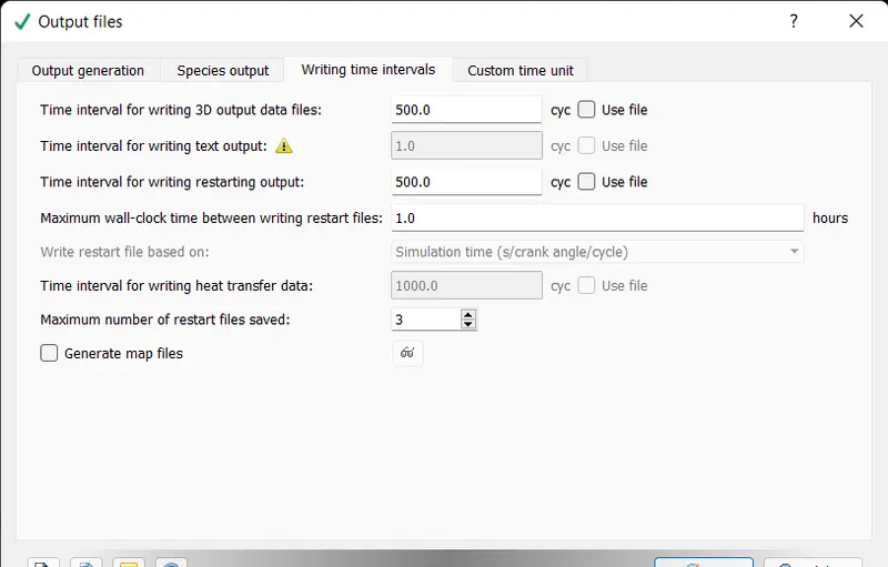
- Output files were selected as per the need
Materials
Simulation parametres
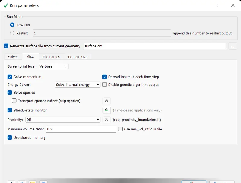
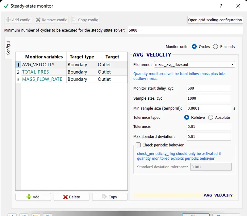
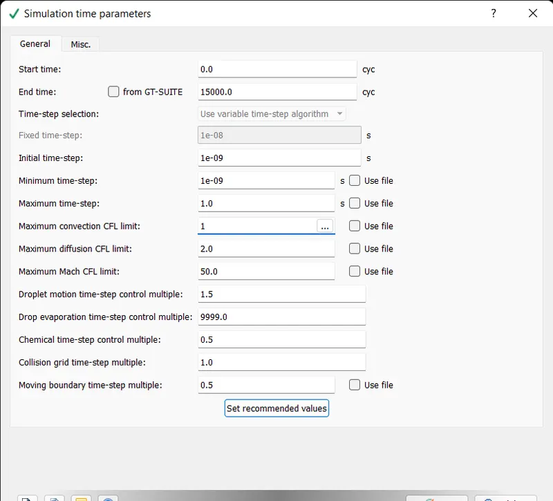
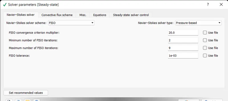
Running the simulation
- Inorder to run the simulation the input files are exported to a specified folder
- Then 'mpiexec.exe' file is copied from the convergent science directory -> converge -> 3.0.16 -> bin -> mpi -> intel64 -> bin
- Also another file named 'converge.exe' is also copied and pasted to the same folder . This file is availible in the Convergent_Science -> CONVERGE -> 3.0.16 -> bin -> msmpi folder
- CYGWIN is run as administrator and navigated to the folder containing the input files
- Then the following command is typed to start the calculation 'mpiexec.exe -n 2 converge.exe restricted'
Post processing
- After running the simulation the output files are availble in the same folder
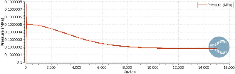
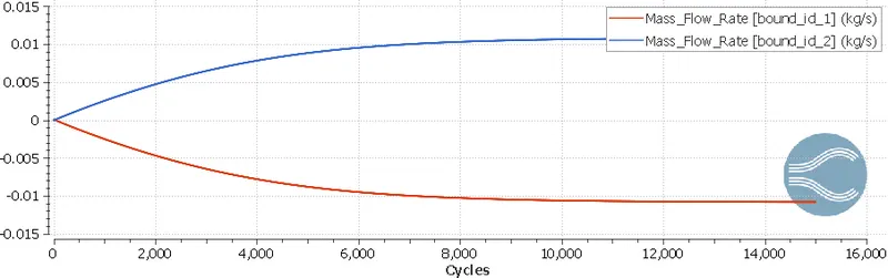
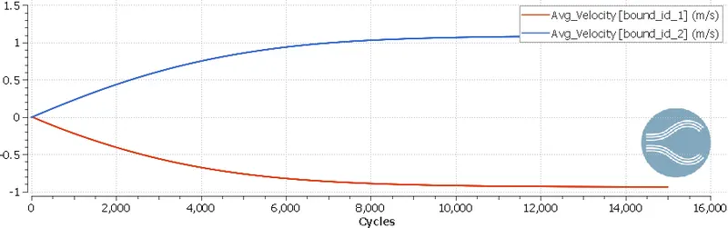
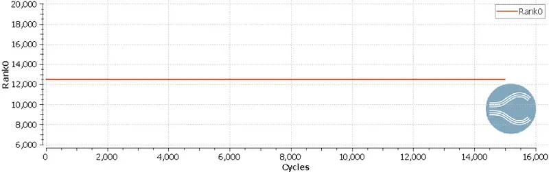
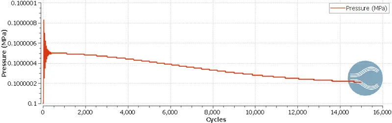
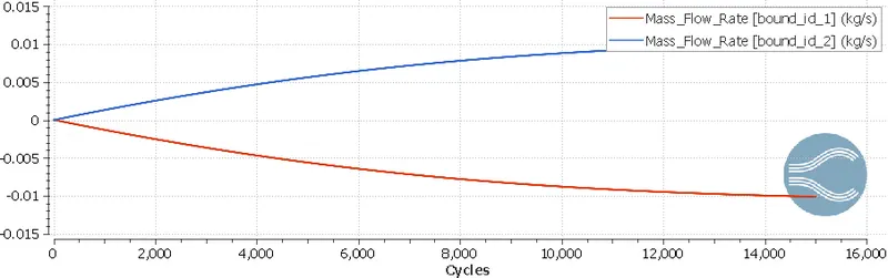
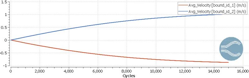
- We can check whether the simulation has converged or not using the convergant studio line plotting, mass flow rate , velocity , pressure at inlet and outlet are obtained here
- For extracting the contour we need 3D files in output folder to be opened through paraview
- So inorder to make the files readable in paraview they are converted to either vtk file or case file. The conversion is done in Post processing in Convergant studio
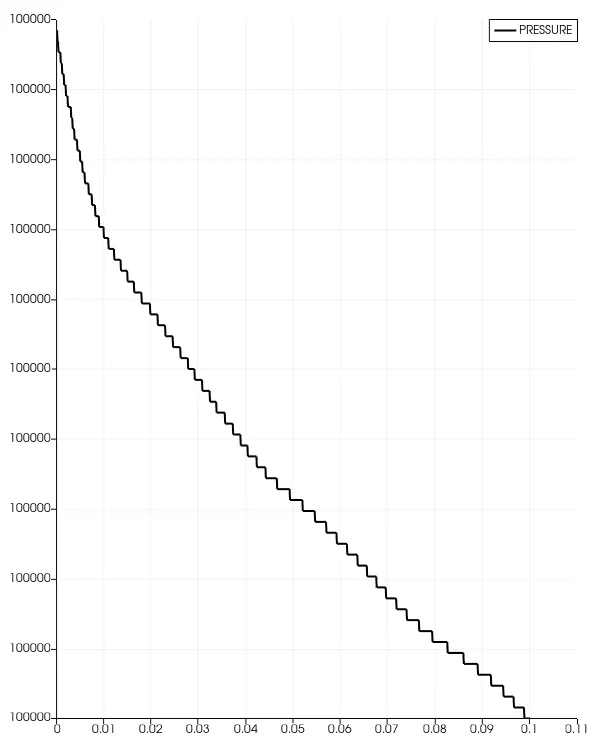
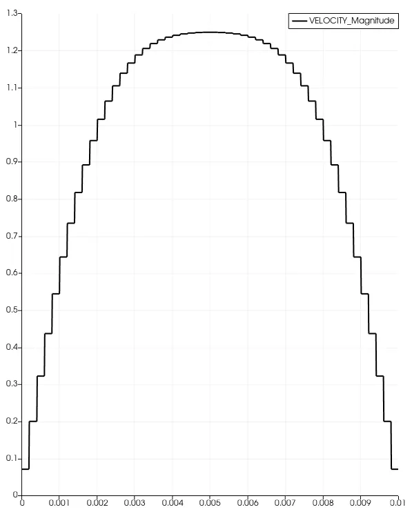
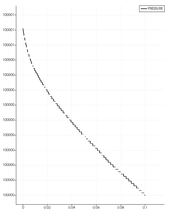
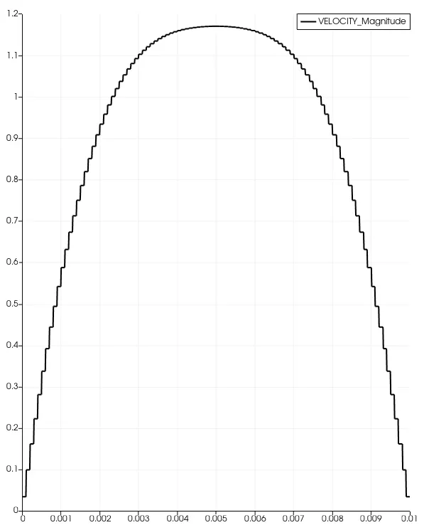
- Plot over line option helps to obtain the plots of pressure drop along the pipe and the velocity variation of flow across the pipe
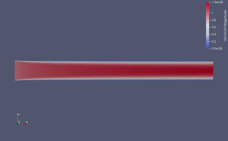
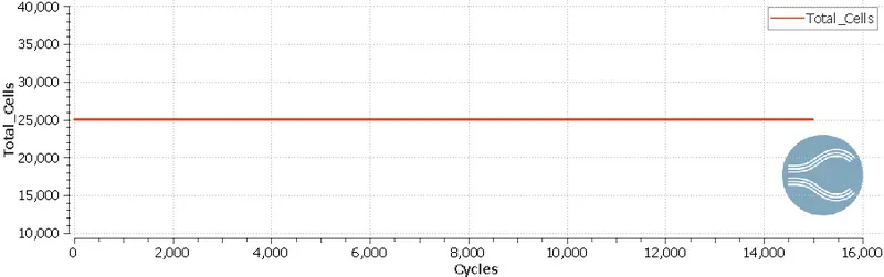
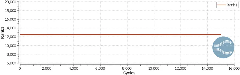
Case1 - Mesh size = 2e-4m
Case2 - Mesh size = 1.5e-4m
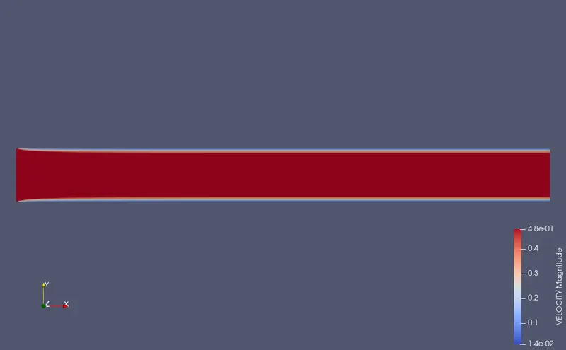
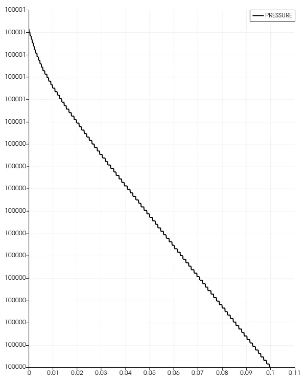
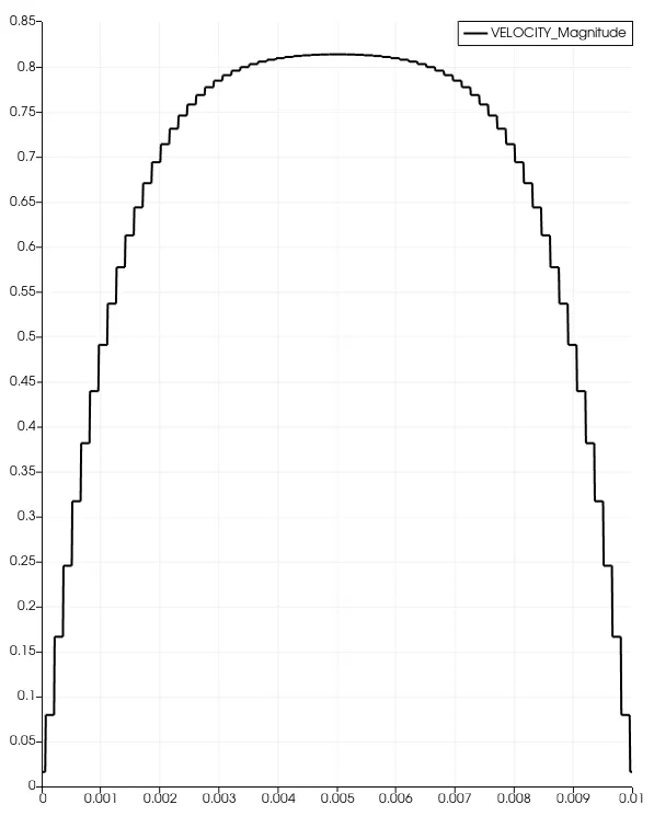
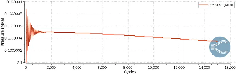
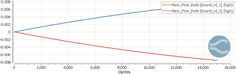
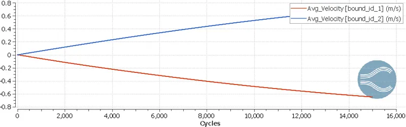
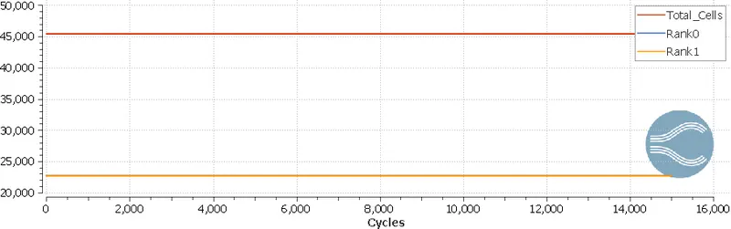
Case3 - Mesh size = 1e-4m
Animations
Case-1
Case-2
Case-3
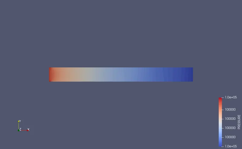
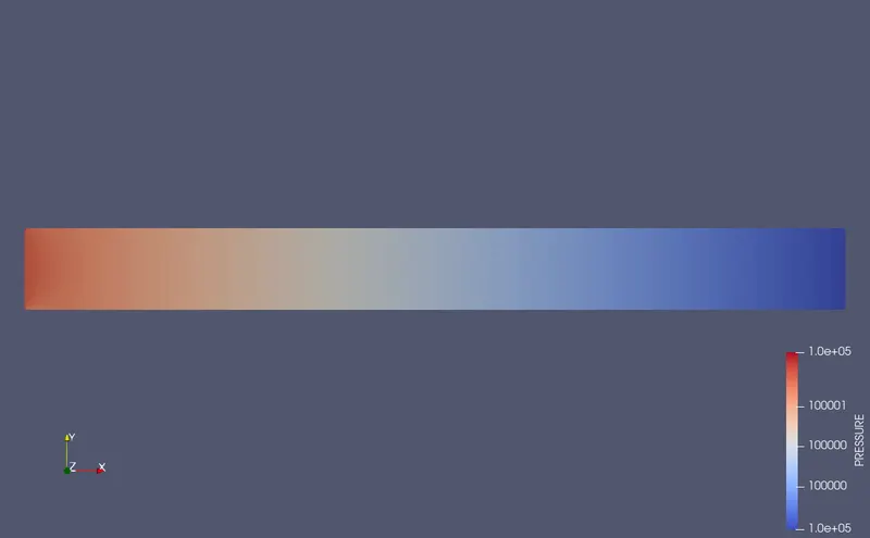
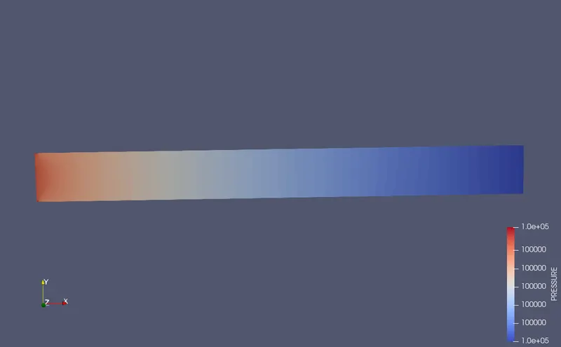
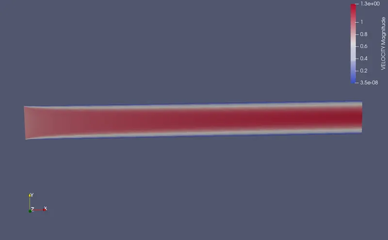
- Since this is steady state study the contour devloped is of a flow that is steady or in other words the devoloped contours is an end result
- The pressure contour is devolped as per the inputs we have given, Since the outlet pressure is lower than the inlet pressure the flow devolopes from inlet to outlet
Observations
- As the mesh size is decreased the solution gets converged at higher number of cycles
- As the mesh is decreased the total cells involved in the simulation increases
- More computation time is required to solve a problem involving more number of cell count
- The values obtained from highly refined mesh is more accurate
- The parabolic variation in the velocity plot across the channel is becouse of the boundary condition given to the walls as 'no slip' condition.
- The plots are much more refined for smaller mesh sizes
- The negetive value in the plots denotes the fluid is leaving the system
- Since the accuracy of case 1 setup is lower, the mesh sizes of case 2 and 3 are preferable
Conclusion