Week 1: Channel flow simulation using CONVERGE CFD
CHANNEL FLOW SIMULATION USING CONVERGE CFD
Aim:-
To simulate the channel flow with three different mesh sizes and shows the contour plots and line plots for different variables.
Introduction:-
Channel flow is an internal flow in which the wall change the hydrodynamic structure of the flow from an arbitrary state at the channel inlet to a certain state at the outlet.
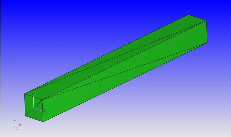
In this simulation, the flow of fluid is in laminar. The 2D geometry has been analysing. Because the cross-section of the geometry is the same. The case setup has been done through converge studio and the simulation is executed using the Cygwing command window. The Post-Processing has been done through Paraview.
Simulation Process.
A. Geometry setup:-
Shape:-
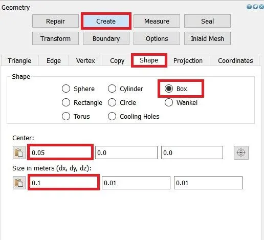
In Converge studio the geometry has been creating using the 'Box' shape under the create option with length 0.1 meter and cross-section of 0.01 X 0.01 metre.
Boundary:-
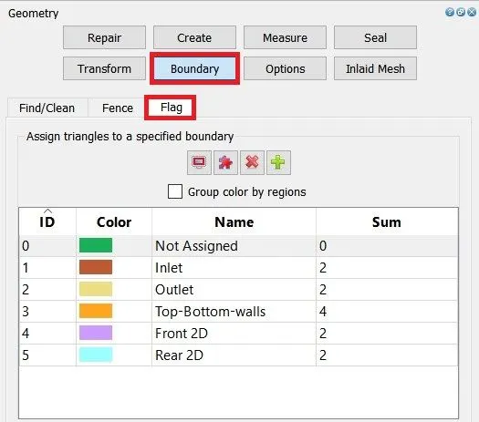
In the Boundary tab, the name of the boundary and the surface has been defined under the Flag option.
Normals:-
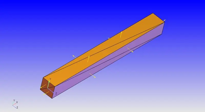
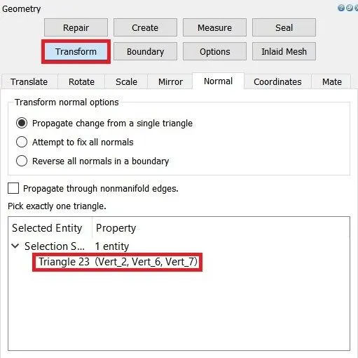
To clear the geometry using the "Normal" which is under the transform tab.
B. Case Setup:-
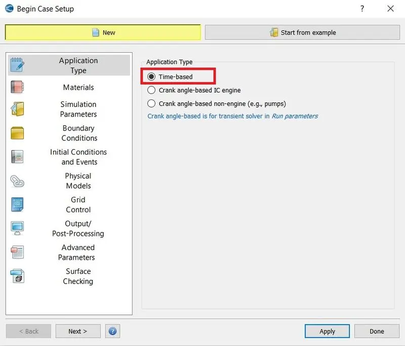
1. Application Type
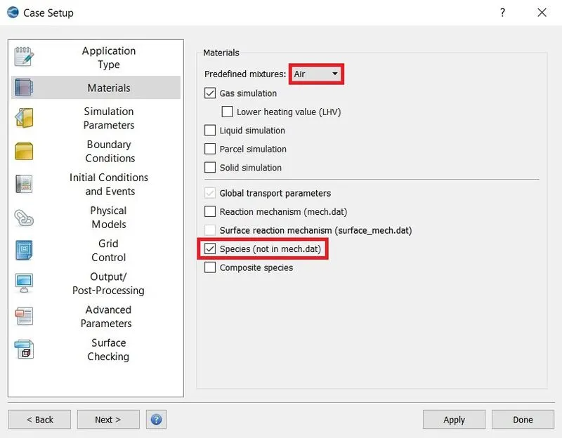
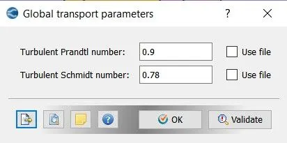
2. Material:-
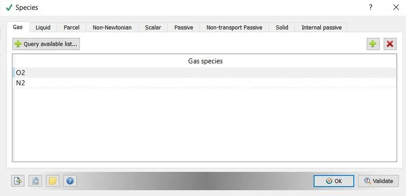
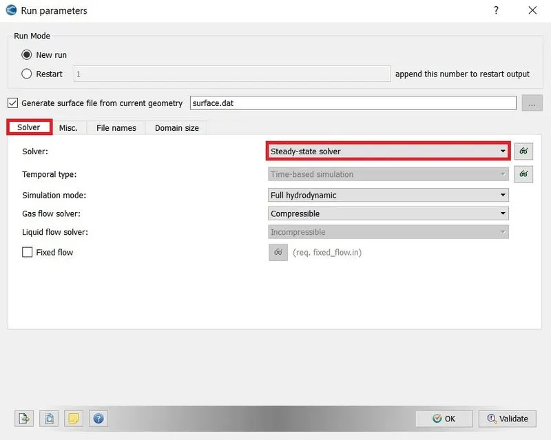
3. Simulation Parameters:-
- A steady-state solver is used.
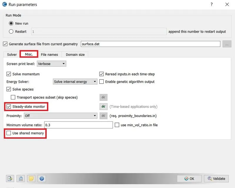
- The steady-state monitor is enabled.
- Use share memory is unchecked.
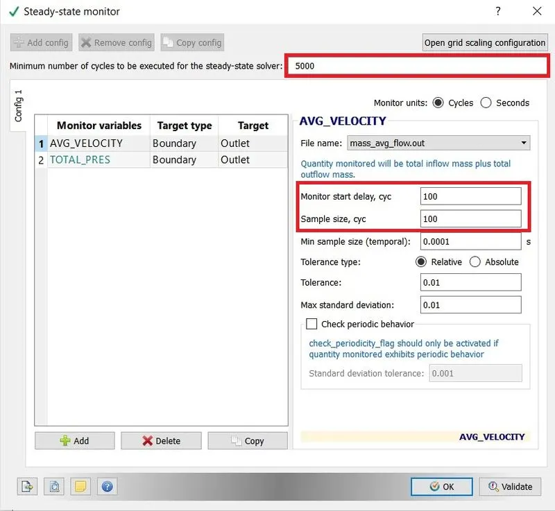
4. Steady-state monitor:-
- Average Velocity and Total Pressure is monitored.
- Minimum number of cycles to be executed for the steady-state solver = 5000
- Monitor start delay and sample size = 100 cycles.
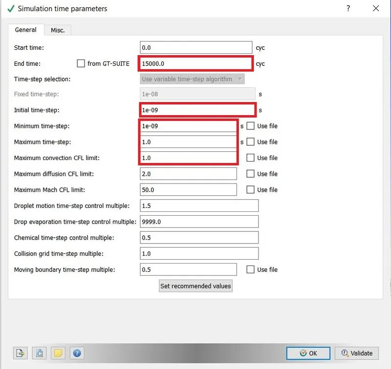
5. Simulation time Parameters:-
6. Solver Parameters:-
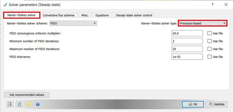
- A pressure-based solver is used.
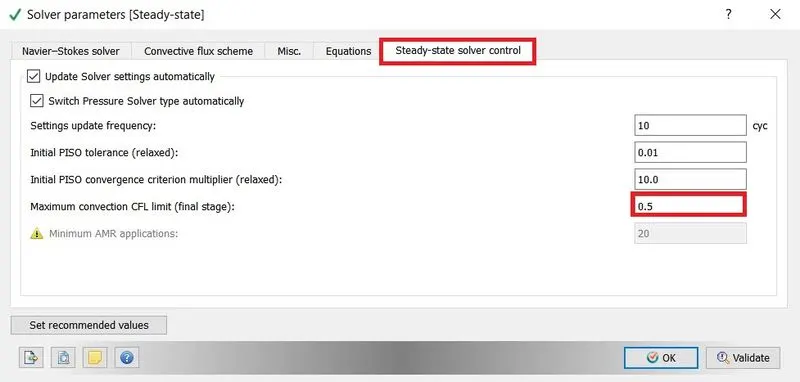
- Maximum CFL limit for final stage is = 0.5
- The preconditioned for pressure equation is set to be "None"
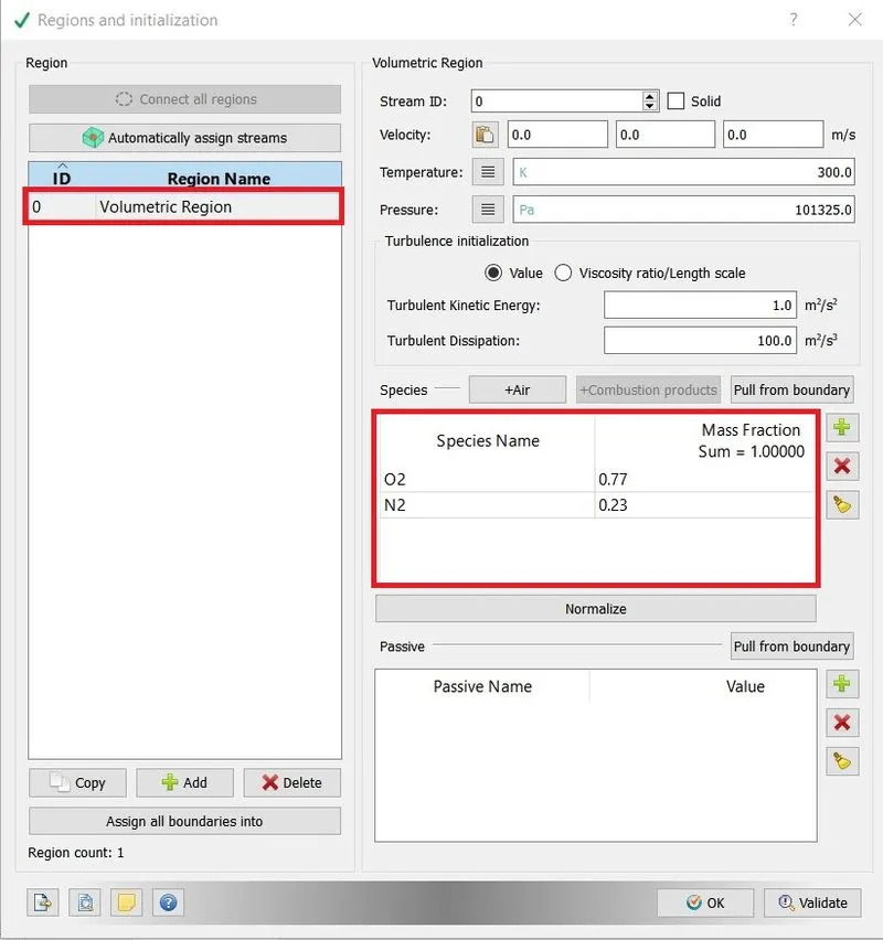
7. Region and Initialization:-
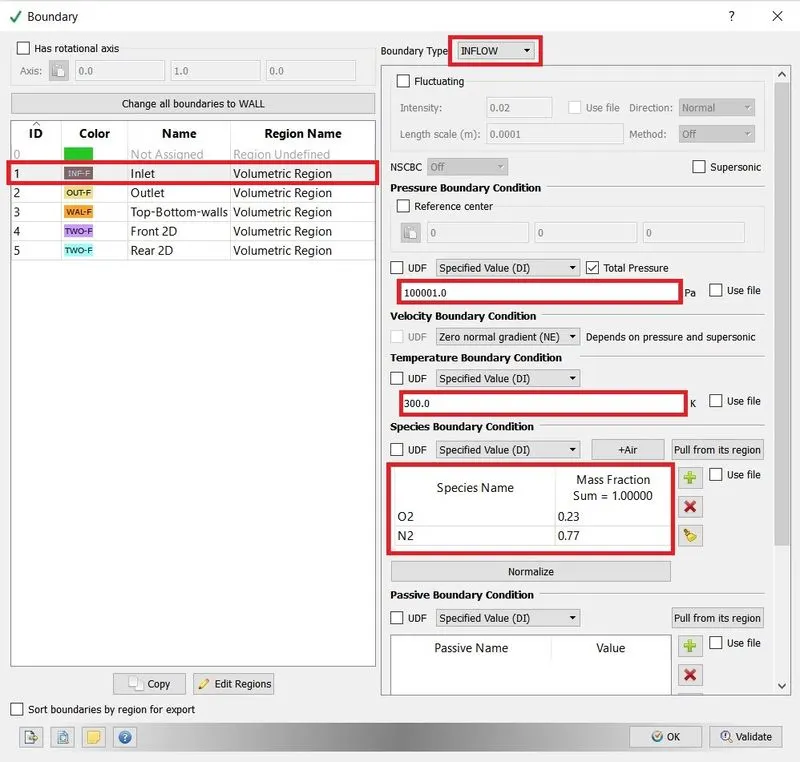
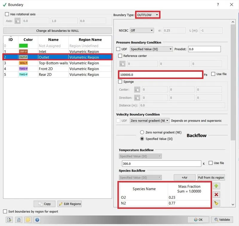
8. Boundary Conditions:-
- Inlet = Inflow with pressure = 100001 [Pas] .
- Outlet = Outflow with pressure = 100000 [Pas].
- Top-Bottom-walls = Wall with no-slip .
- Front 2D = Two_D
- Rear 2D = Two_D
All the boundary condition is assigned with the volumetric region.
9. Grid Control:-
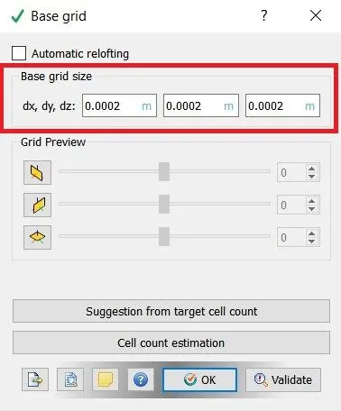
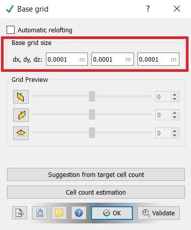
The base mesh for 3 cases is
| Case_1 | dx=0.0002 m | dy=0.0002 m | dz=0.0002 m |
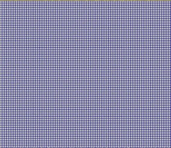
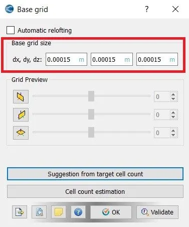
| Case_2 | dx=0.00015 m | dy=0.00015 m | dz=0.00015 m |
| Case_3 | dx=0.0001 m | dy=0.0001 m | dz=0.0001 m |
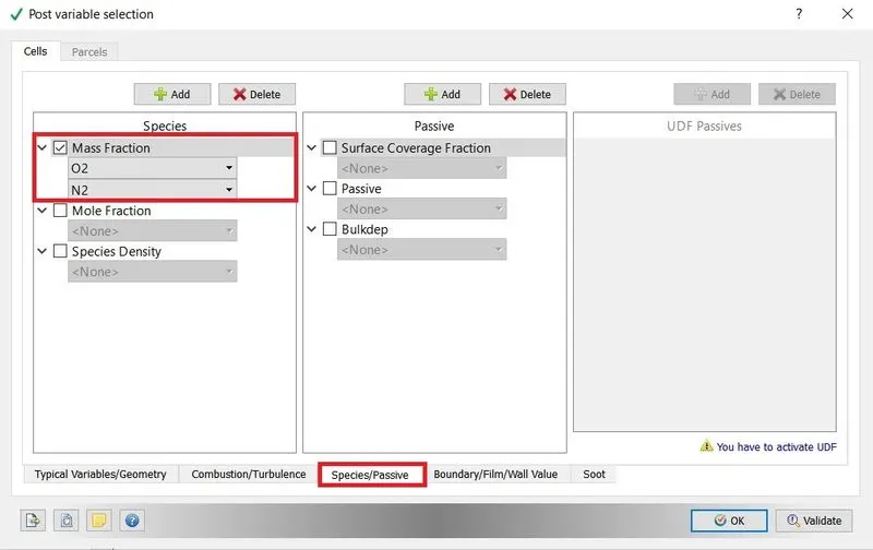
10. Output /Post-processing:-
Post variable selection = Enable Mass fraction of O2 and N2.
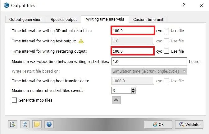
Output files for time intervals.
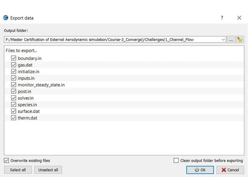
11. Export Data:-
Export all the input files to run the simulation in Cygwin.
*****************************************************************************
CASE - 1
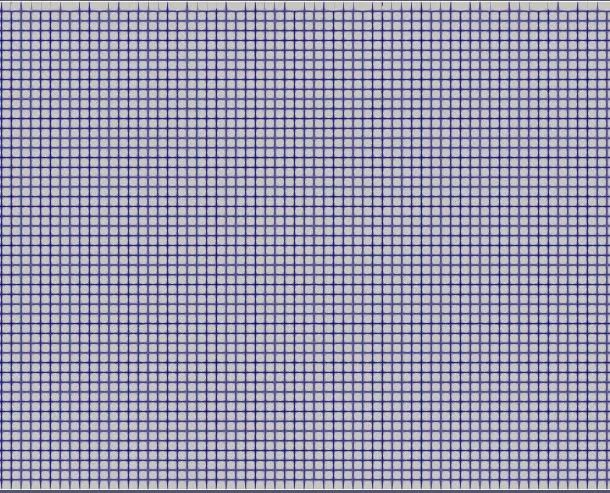
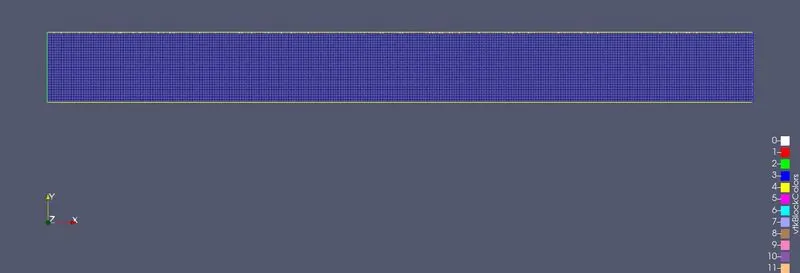
Mesh:-
Execute the Simulation:-
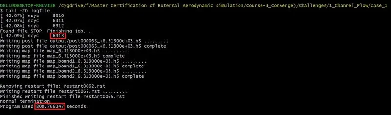
To run the simulation in Cygwin using the command.
mpiexec.exe -n 4 converge.exe restricted </dev/null> logfile &
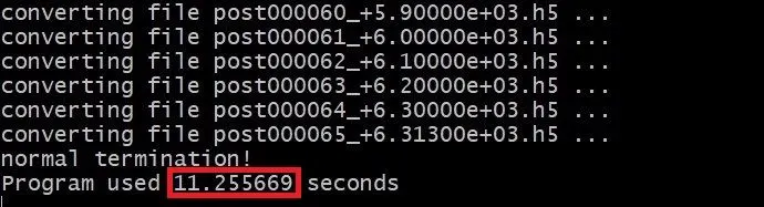
After the simulation is complete, it can be converted into Paraview VTK in-line binary Format to post-process the result in ParaView.
mpiexec.exe -n 4 post_convert_30_msmpi.exe
Post Processing Result:-
1. Contour.
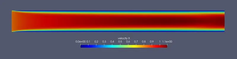
Fig(a). Velocity Contour
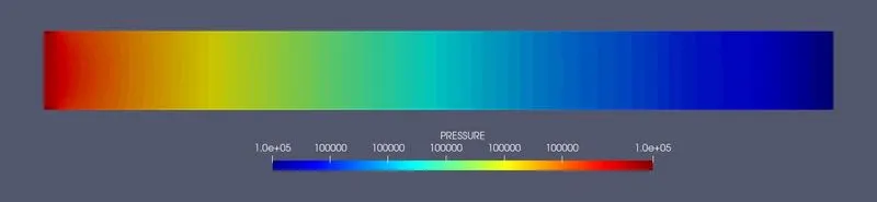
Fig(b). Pressure Contour
2. Velocity Plot from Paraview.
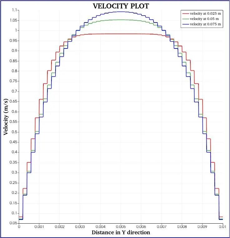
From the plot, the velocity is measured at different locations of the channel (0.025m, 0.05m, 0.075m) in the base mesh of 0.0002m. The Laminar flow has a parabolic curve and it is achieved at the fully developed region of the channel.
3. Line Plot from Converge:-
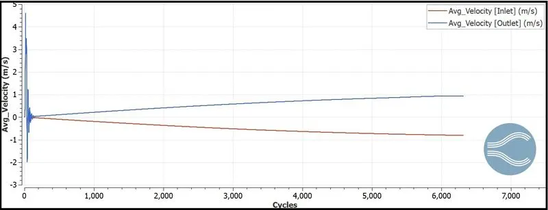
Fig(a). Average Velocity
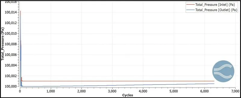
Fig(b). Total Pressure
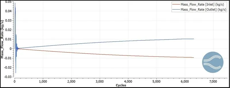
Fig(c). Mass Flow Rate
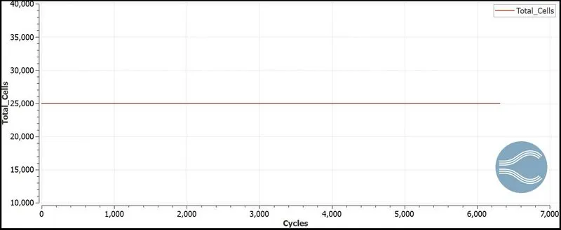
Fig(d). Total cells
4. Animation:-
Link:- Channel Flow Animation of mesh size 0.0002m.
*****************************************************************************
CASE - 2
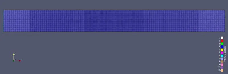
Mesh:-
Execute the Simulation:-
To run the simulation in Cygwin using the command.
mpiexec.exe -n 4 converge.exe restricted </dev/null> logfile &
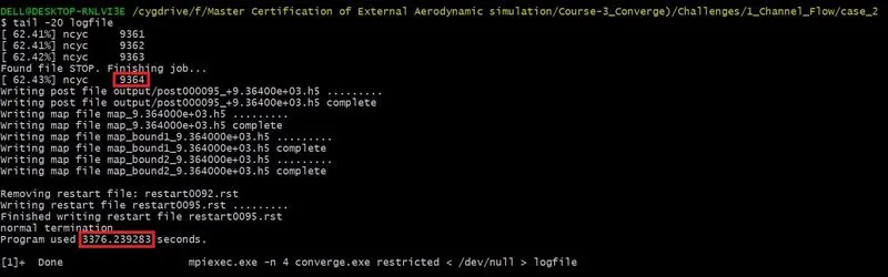
After the simulation is complete, it can be converted into Paraview VTK in-line binary Format to post-process the result in ParaView.
mpiexec.exe -n 4 post_convert_30_msmpi.exe
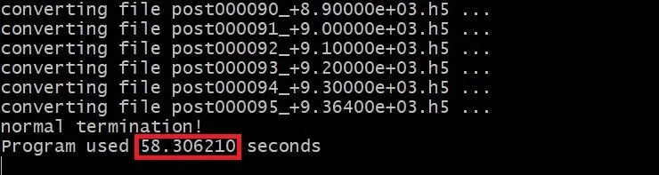
Post Processing Result:-
1. Contour.
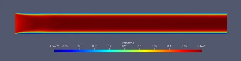
Fig(a). Velocity Contour
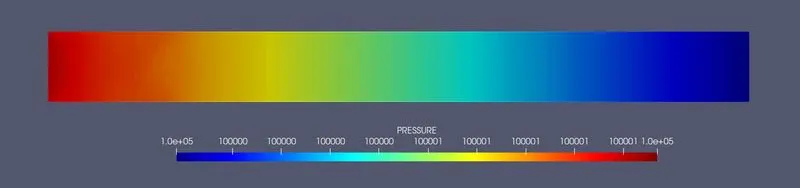
Fig(b). Pressure Contour
2. Velocity Plot from Paraview.
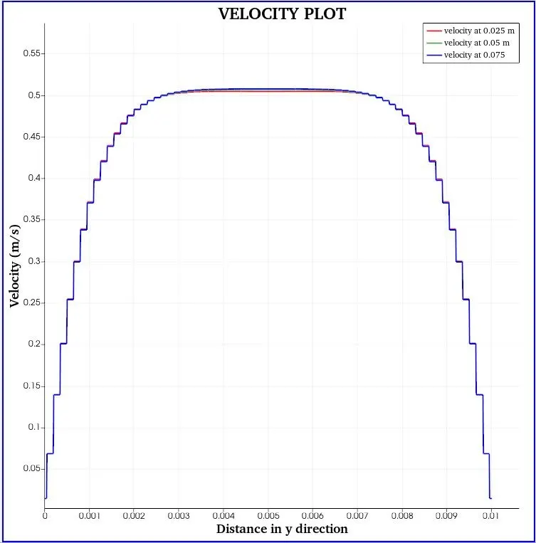
From the plot, the velocity is measured at different locations of the channel (0.025m, 0.05m, 0.075m) in the base mesh of 0.00015m. The Laminar flow has a parabolic curve and it is achieved at the fully developed region of the channel.
3. Line Plot from Converge:-
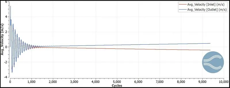
Fig(a). Average Velocity
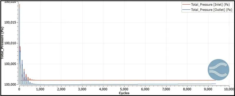
Fig(b). Total Pressure
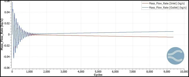
Fig(c). Mass Flow Rate
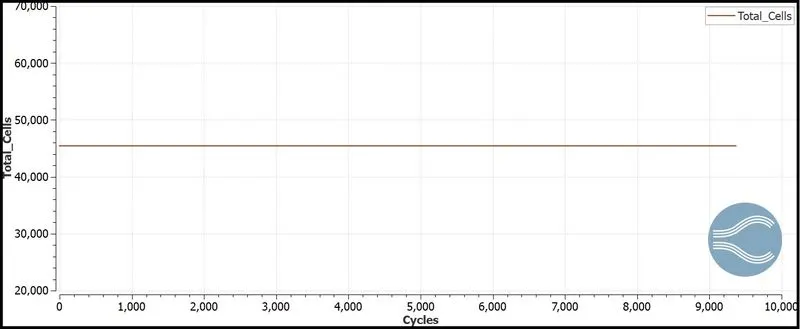
Fig(d). Total cells
4. Animation:-
Link:- Channel Flow Animation of base mesh 0.00015m.
*****************************************************************************
CASE - 3
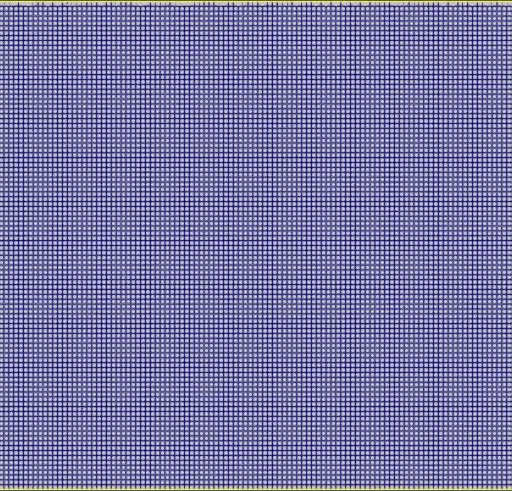
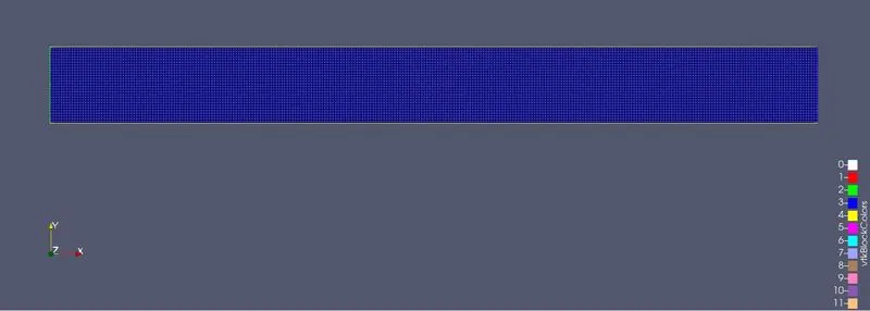
Mesh:-
Execute the Simulation:-
To run the simulation in Cygwin using the command.
mpiexec.exe -n 4 converge.exe restricted </dev/null> logfile &
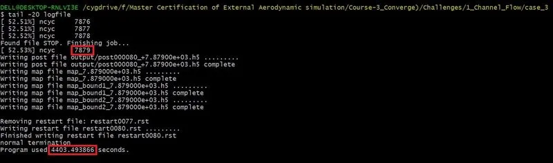
After the simulation is complete, it can be converted into Paraview VTK in-line binary Format to post-process the result in ParaView.
mpiexec.exe -n 4 post_convert_30_msmpi.exe
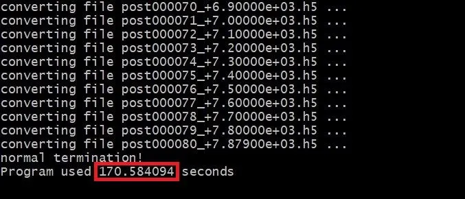
Post Processing Result:-
1. Contour.
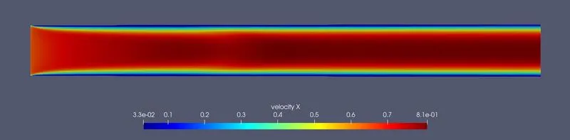
Fig(a). Velocity Contour
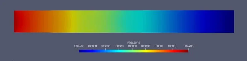
Fig(b). Pressure Contour
2. Velocity Plot from Paraview.
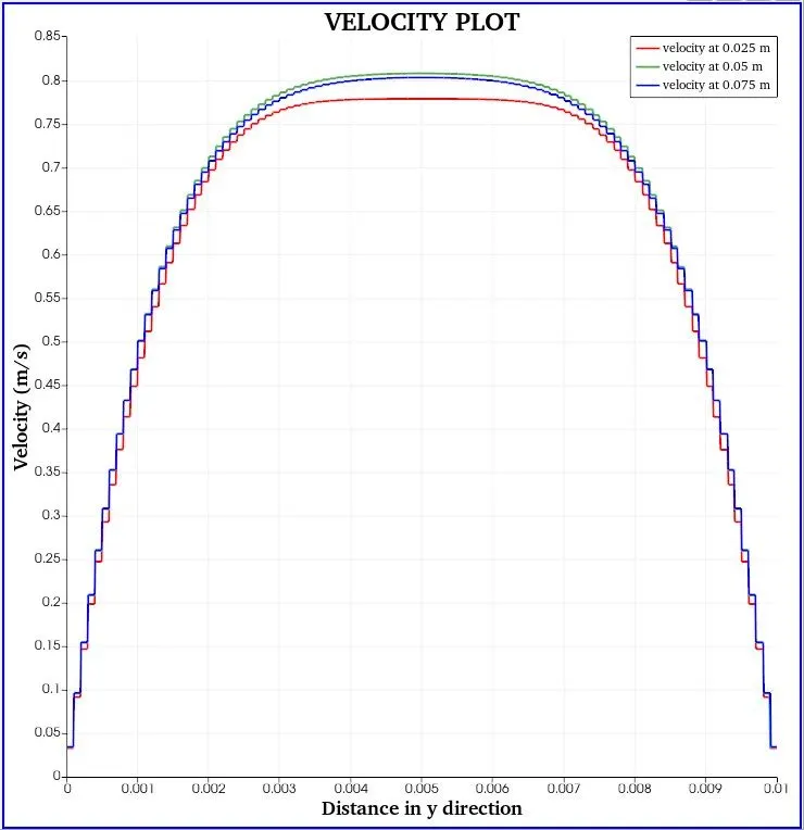
From the plot, the velocity is measured at different locations of the channel (0.025m, 0.05m, 0.075m) in the base mesh of 0.0001m. The Laminar flow has a parabolic curve and it is achieved at the fully developed region of the channel.
3. Line Plot from Converge:-
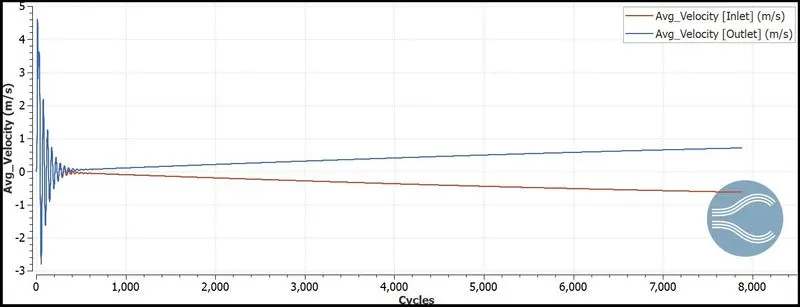
Fig(a). Average Velocity
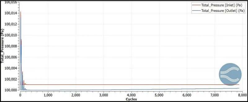
Fig(b). Total Pressure
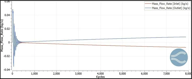
Fig(c). Mass Flow Rate
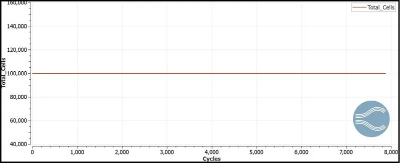
Fig(d). Total cells
4. Animation:-
Link:- Channel Flow Animation of mesh size 0.0001m.
Conclusion:-
- The velocity plot from ParaView shows that if the cell count is increased the velocity profile looks like a perfect parabolic curve at the fully developed region. In the hydrodynamic entrance region, the velocity profile is in a developing region.
- In the Pressure plot, the pressure is constant with respect to the number of cycles.
- In the mass flow rate plot, the out mass flow rate is negative because it shows the fluid is discharging from the domain.
- The Total cell count plot shows the total cells count remains constant. This represents there is no loss or gain of cells in the simulation.
- This simulation shows the basic flow of fluid and different variables in the domain.