Week 1: Channel flow simulation using CONVERGE CFD
CHANNEL FLOW SIMULATION USING CONVERGE CFD
AIM: to run 3 channel flow simulations and compare the results between all the 3 simulations based on grid Mesh.
OBJECTIVE:
1. Velocity and pressure contours for all the 3 base mesh sizes
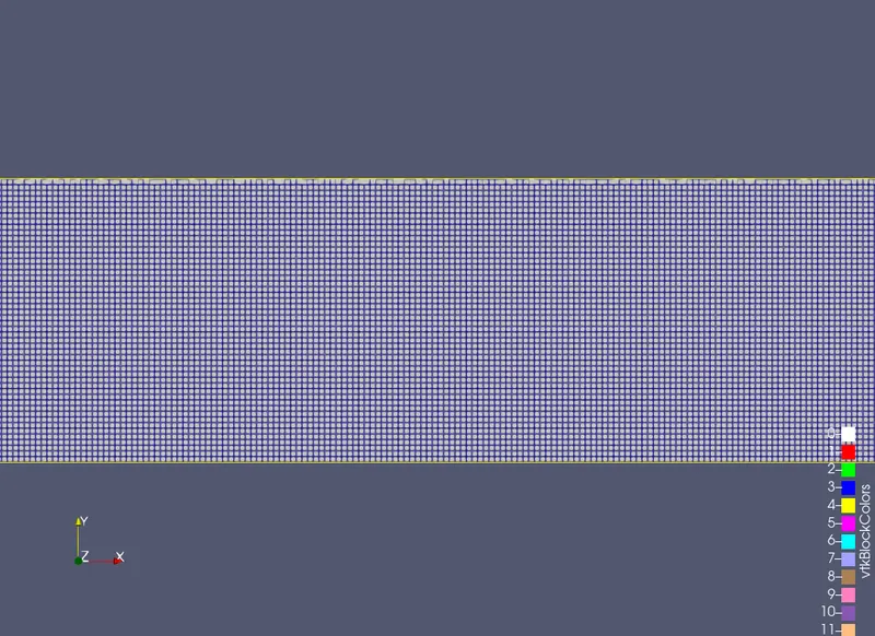
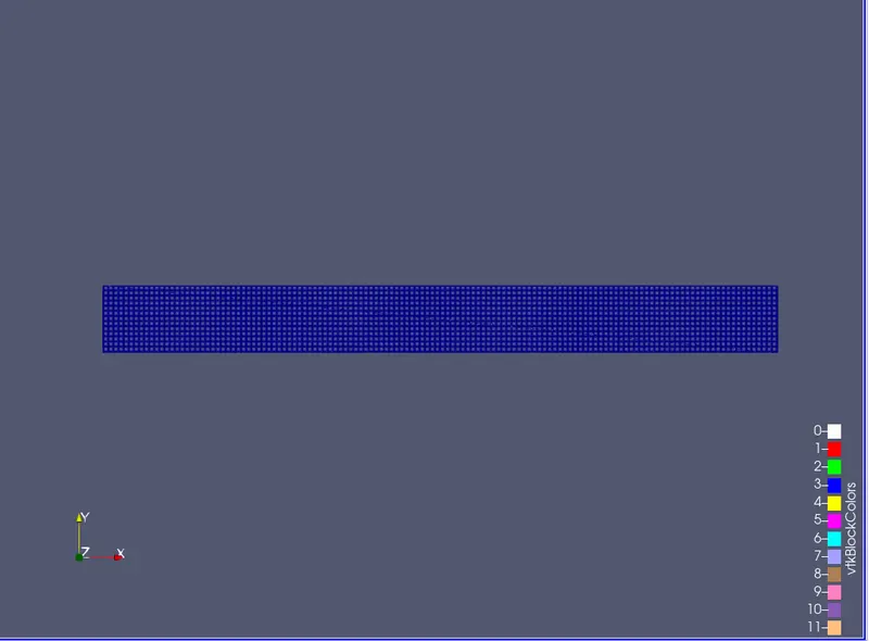
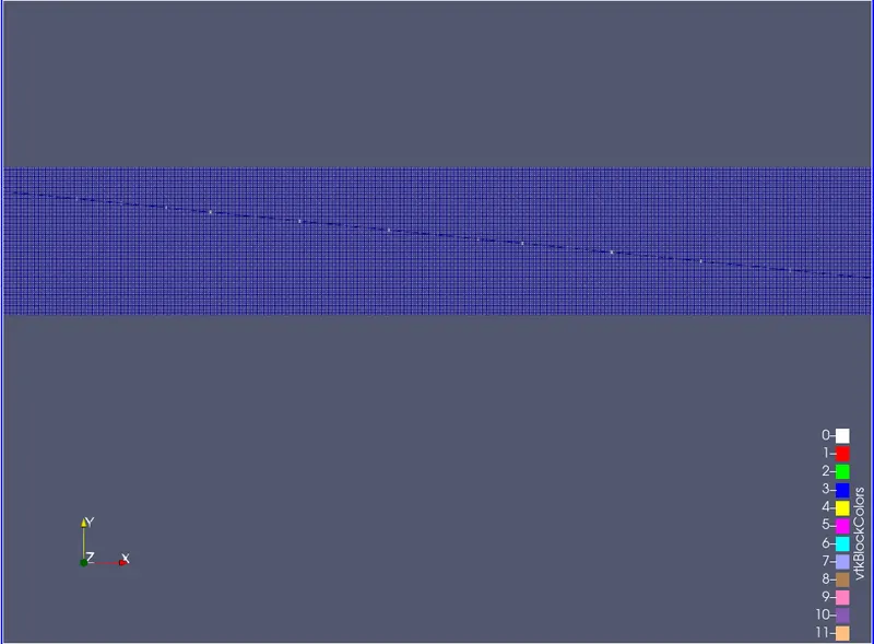
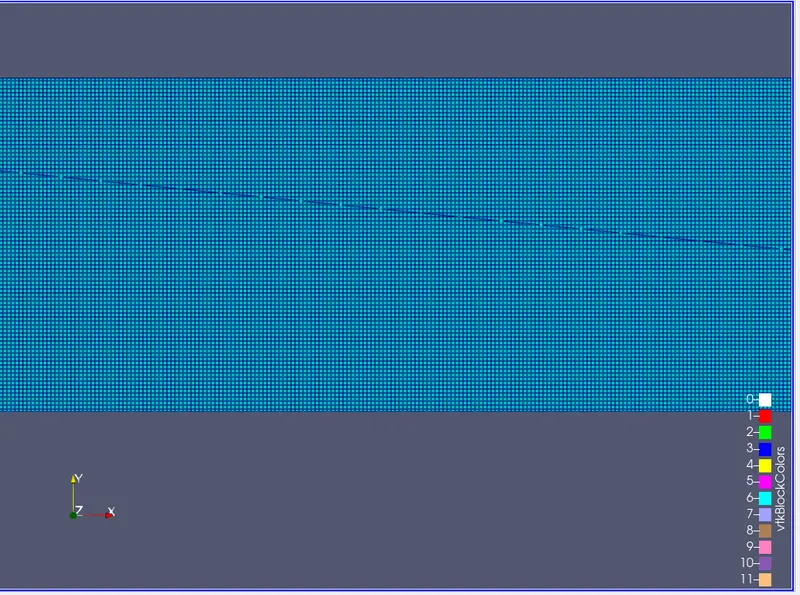
2. Show mesh (i.e surface with edges) for the 3 base mesh sizes
3. Plots for velocity, pressure, mass flow rate, and total cell count for all 3 base mesh sizes.
4. Explain the plots and write a detailed report on your project.
5. Upload an animation to youtube and attach the link here using the add media option. Explain the development of the flow using the animation.
THEORY:
The results of a CFD simulation are obtained by solving the Navier-Stokes equations. These are 5 equations, continuity, momentum (3 equations), and energy equations. The continuity and momentum equations are solved for all types of flow problems and the energy equation can be used only when heat transfer is taking place to speed up the simulation. These equations are numerically solved in computers using algorithms like SIMPLE and PISO.
We assume that there is no heat transfer happening and the flow is incompressible. So we have 4 equations (Continuity and 3 momentum equation) to solve and 4 unknowns (Pressure and Velocity in 3 directions).
Continuity Equation:
`{delu}/{delx} + {delv}/{dely} +{delw}/{delz} =0`
X-Momentum
`rho{Du}/{Dt} = -{delp}/{delx} + munabla^2u + pf_x`
Y-Momentum
`rho{Dv}/{Dt} = -{delp}/{dely} + munabla^2v + pf_y`
Z-Momentum
`rho{Dw}/{Dt} = -{delp}/{delz} + munabla^2w + pf_z`
Where u, v and w are the velocities in x, y and z directions respectively
`rho` is the density and p is the pressure, `nabla = del/{delx} + del/{dely} +del/{delz}`
These equations are solved using the pressure correction method by using the SIMPLE and PISO algorithms.
Here we can see that all 4 equations have a velocity term and only 3 equations have a pressure term so we need to use the pressure correction method.
SIMULATION AND SOLUTION:
In this project, we simulate 3 cases for 3 different meshes of a channel flow. They are:
- dx = 2e-4m, dy = 2e-4m, dz = 2e-4m
- dx = 1.5e-4m, dy = 1.5e-4m, dz = 1.5e-4m
- dx = 1.2e-4m, dy = 1.2e-4m, dz = 1.2e-4m
Geometry:
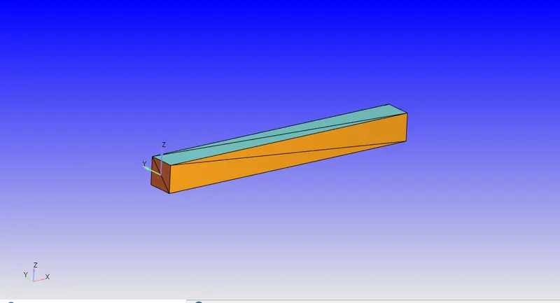
We create a box with dimensions
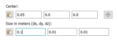
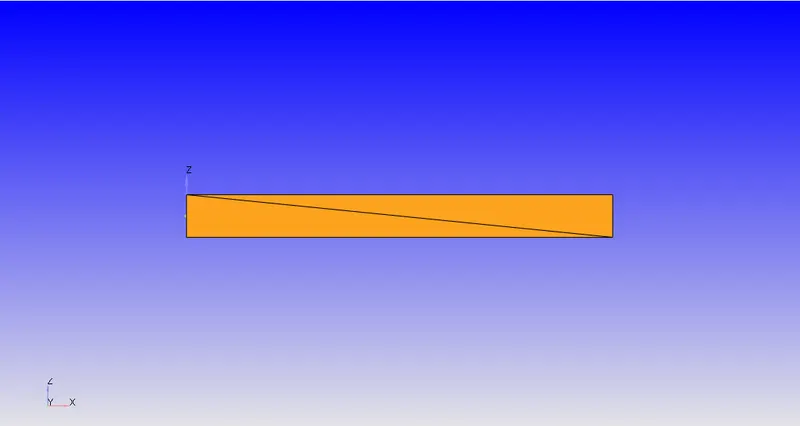
After creating we point the Normal towards the flow.
Setup:
Part 1:
|
SETUP |
|
|
Application Type |
Time-based |
|
MATERIALS: |
|
|
1. Gas simulation |
Standard |
|
2. Global Transport Parameters |
Standard |
|
3. Species |
N2 and O2 |
|
SOLUTION PARAMETERS |
|
|
1. Run Parameters Steady-state monitor: |
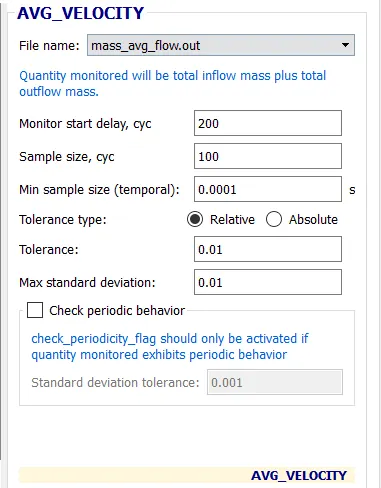
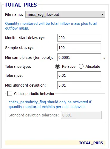
Steady-state solver>Full hydrodynamic>Compressible AVG_Velocity
TOTAL_Pressure
|
|
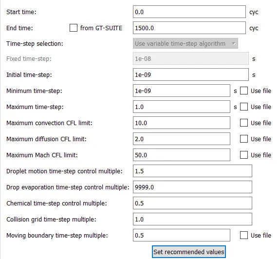
2. Simulation time parameters |
|
|
3. Solver parameters |
Navis-stokes solver scheme: PICO Navis-stokes solver type: Density-based Max convection CFL limit: 0.5 |
|
BOUNDARY CONDITIONS |
|
|
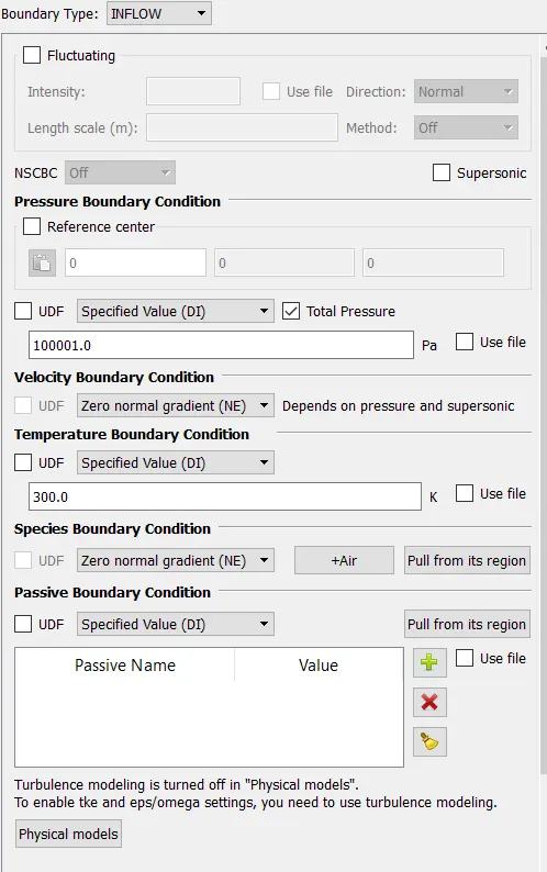
1. Inlet |
 |
|
2. Outlet |
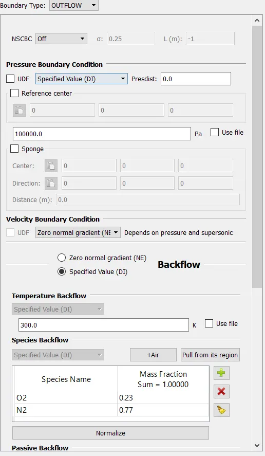 |
|
3. Top and bottom wall |
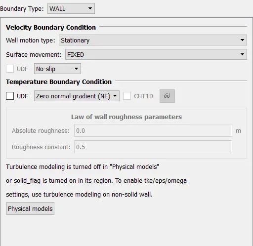 |
|
4. Front wall |
2-D Wall |
|
5. Back wall |
2-D wall |
|
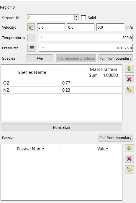
INITIAL CONDITIONS AND EVENTS |
|
|
1. Regions and initialization |
|
|
PHYSICAL MODELS |
Standard |
|
GRID CONTROL |
|
|
1. Base mesh |
3 cases Case 1: dx = 2e-4m, dy = 2e-4m and dz = 2e-4m Case 2: dx = 1.5e-4m, dy = 1.5e-4m and dz = 1.5e-4m Case 3: dx = 1.2e-4m, dy = 1.2e-4m and dz = 1.2e-4m |
|
OUTPUT/POST-PROCESSING |
|
|
1. Post variable selection |
Species/Passive: N2 and O2 |
|
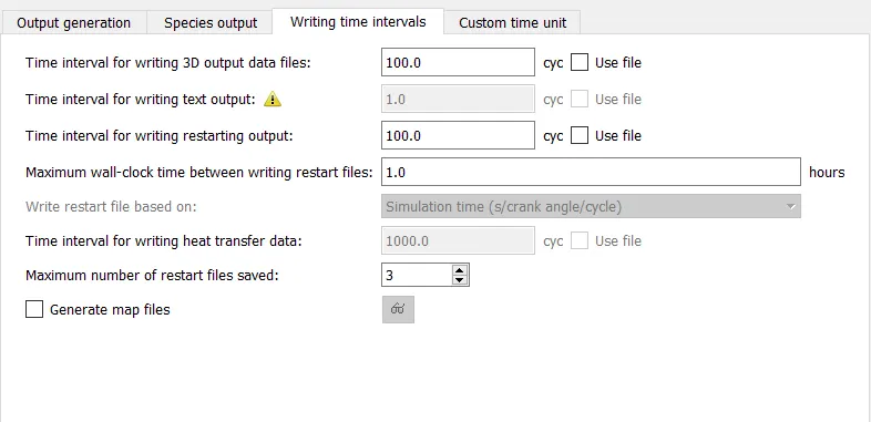
2. Output files: |
|
Mesh:
3 cases
Case 1: dx = 2e-4m, dy = 2e-4m and dz = 2e-4m
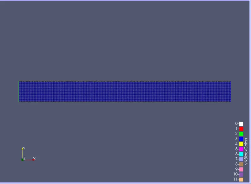
Case 2: dx = 1.5e-4m, dy = 1.5e-4m and dz = 1.5e-4m
Case 3: dx = 1.2e-4m, dy = 1.2e-4m and dz = 1.2e-4m
Solution:
Case 1: dx = 2e-4m, dy = 2e-4m and dz = 2e-4m
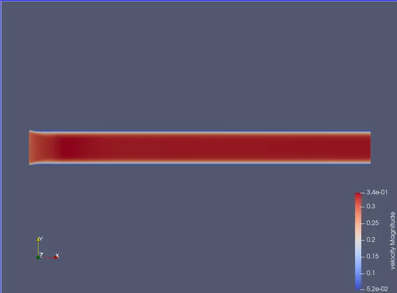
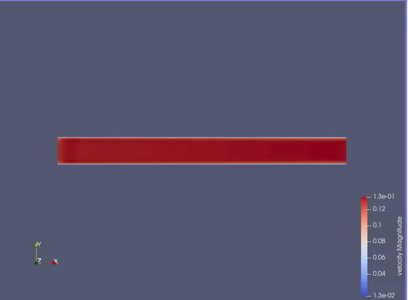
Velocity plot:
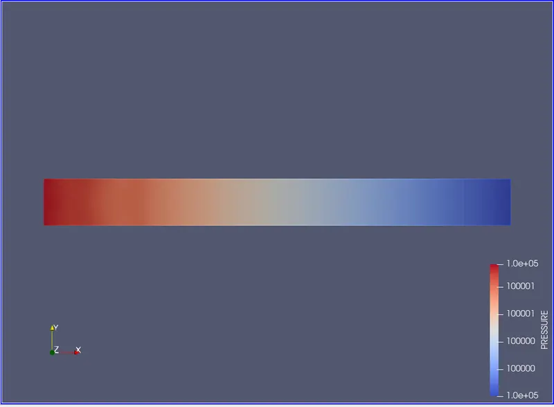
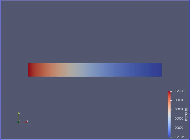
Pressure plot:
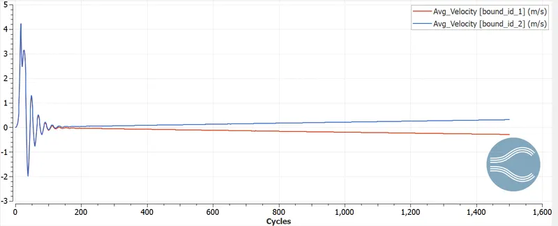
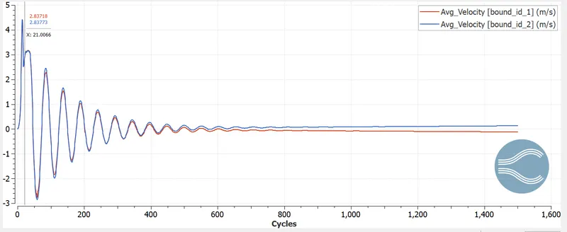
Avg_velocity
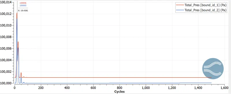
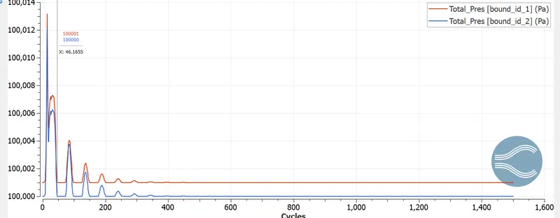
Total_pressure
Mass flow rate:
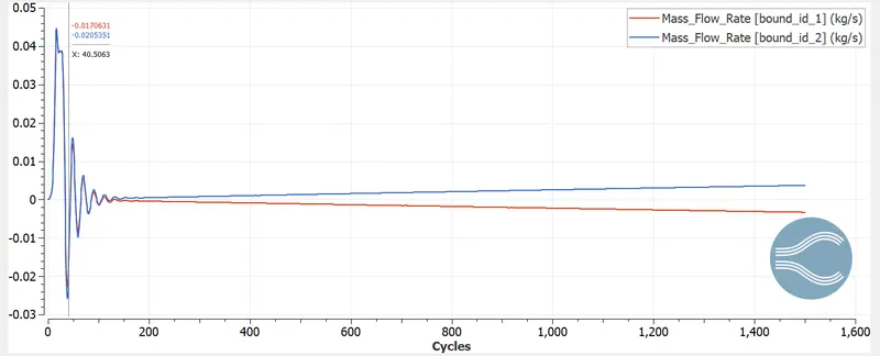
Cell Count
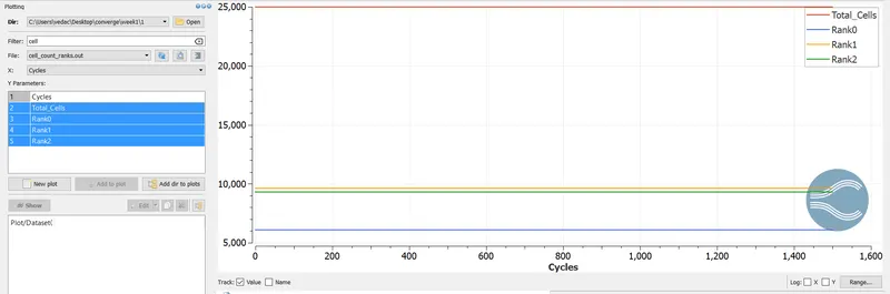
Animation
Velocity:https://youtu.be/0KsGlKAkiM4
Pressure:https://youtu.be/iOkjBseLlH8
Case 2: dx = 1.5e-4m, dy = 1.5e-4m and dz = 1.5e-4m
Velocity plot:
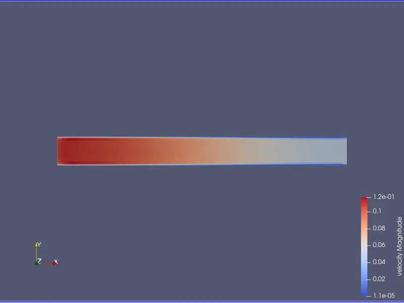
Pressure plot:
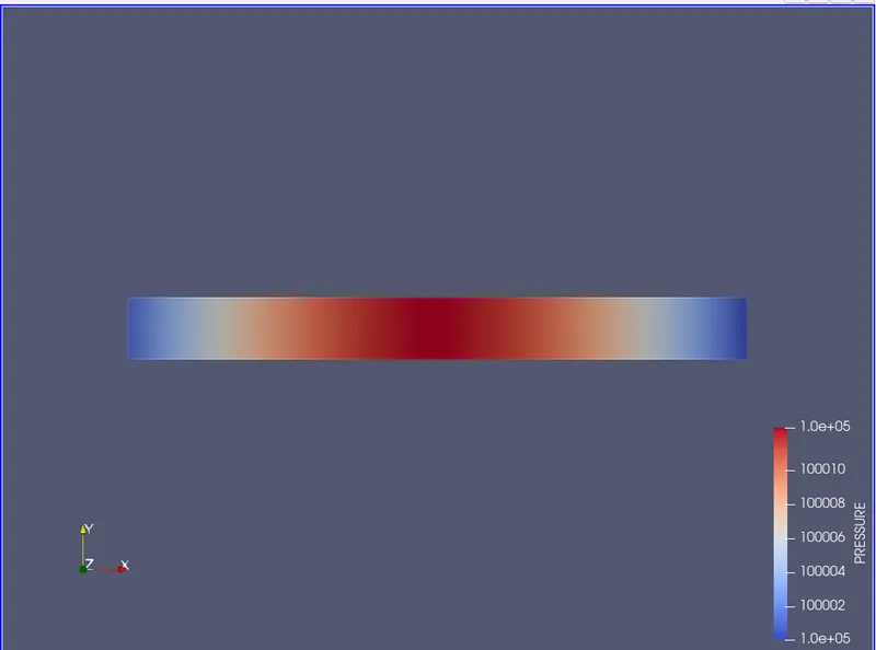
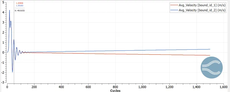
Avg_velocity
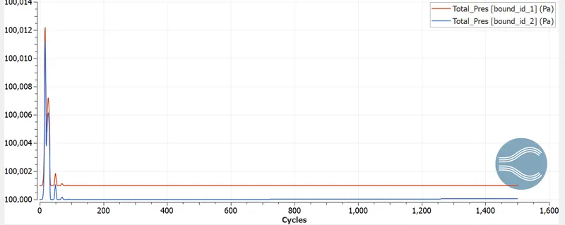
Total_pressure
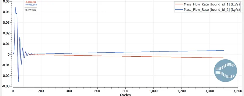
Mass flow rate:
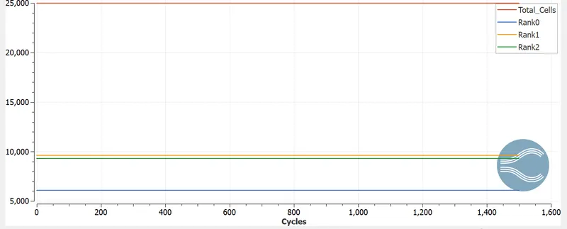
Cell Count:
Animation
Velocity: https://youtu.be/SWlZKeZnSso
Pressure: https://youtu.be/_wnk7lxomGI
Case 3: dx = 1.2e-4m, dy = 1.2e-4m and dz = 1.2e-4m
Velocity plot:
Pressure plot:
Avg_velocity
Total_pressure
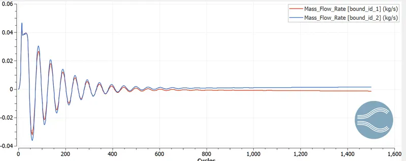
Mass flow rate:
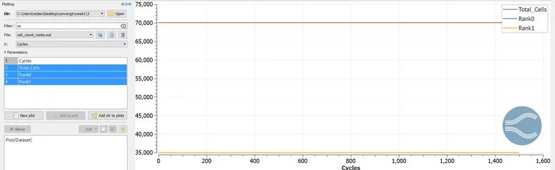
Cell Count
Animation
Velocity:https://youtu.be/1OK2wFJDykg
Pressure:https://youtu.be/9kSKss1Blgs
CONCLUSION:
1. As we decrease the mesh size, the results become more accurate and it produces smooth plots but the computation time increases drastically.
2. As we decrease the mesh size, Converge decreases the time step as well to maintain the CFL number and to keep the solution stable. Because of that the number of cycles required for convergence increases which again increases the computation time.