Week 1: Channel flow simulation using CONVERGE CFD
- Aim - Channel flow simulation using CONVERGE CFD
- Objective
- Setup channel flow simulation.
- Run simulation for 3 different mesh sizes.
- Plot velocity and pressure contours for all 3 mesh sizes.
- Show plots for velocity, pressure, mass flow rate, and total cell count for all 3 mesh sizes.
-
Introduction
- Channel Flow
- A channel flow is an internal flow in which the boundary walls change the hydrodynamic structure of the flow from an arbitrary state at the channel inlet to a specific state at the outlet.
- There are three types of fluid flow: laminar, turbulent and transitional.
- The conditions leading to each flow behavior are system specific.
- Open Channel Flow Types
Steady and unsteady flows.
Uniform and uneven flow.
Laminar and turbulent flow. - The simplest representation of internal flow is laminar flow in a circular tube, but turbulent flow in the rotor of a centrifugal compressor is the most complex example of internal flow. Engineering equipment uses ducts with cross-sections of various geometric shapes.
- This project used Converge Studio to establish a working idea of simulating airflow through a duct flow under certain parameters. This is systematically detailed in this report.
- Procedure
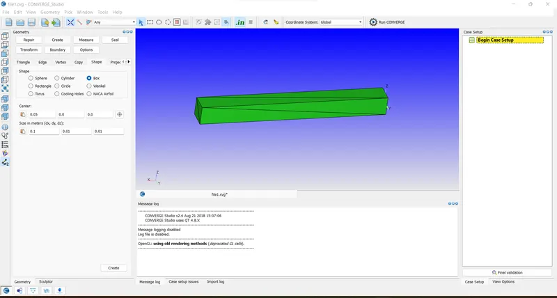
- Creating a geometry using the creation tool of Converge Studio
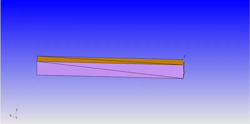
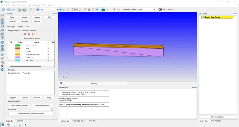
- Setting up boundries
-
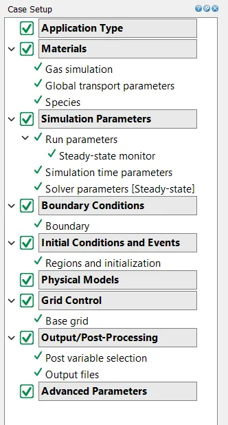
Case Setup:
- Application Type = Time-based
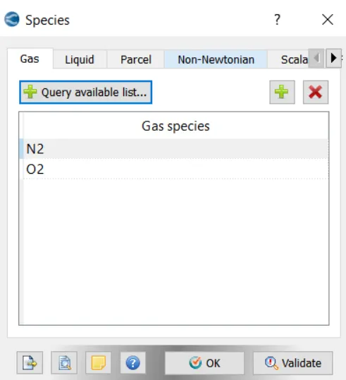
- Materials- Air
- Gas simulation is checked. The species are O2 and N2.
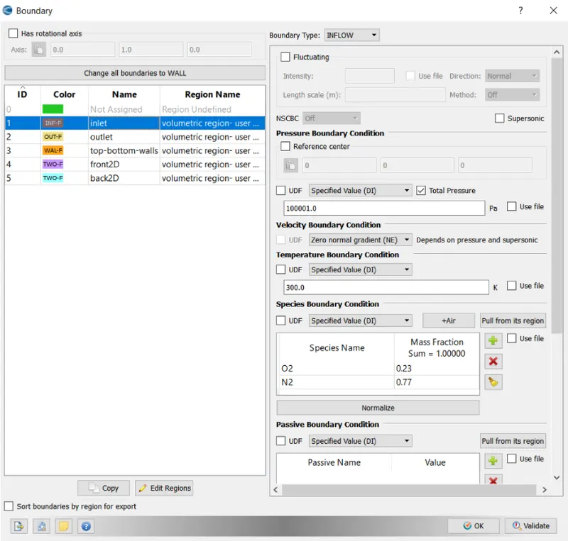
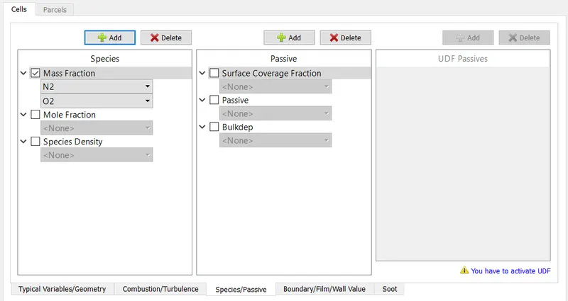
- Post Variable Selection:
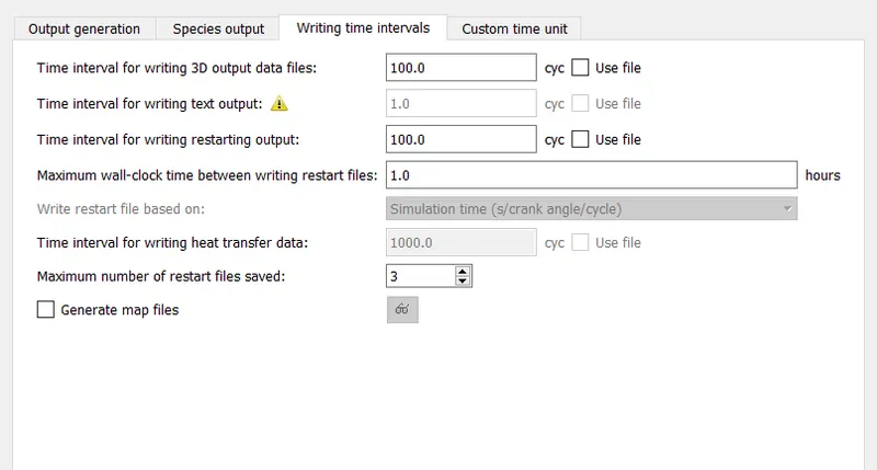
- Output Files:
- Once the case setup is complete, all input files will be exported to a specific folder
- Cygwin is then used to resolve the inputs, and once the simulation is complete, the resulting data converges into a format readable by Paraview.
Post-processing is done in Paraview. - Results
- Grid Size
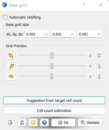
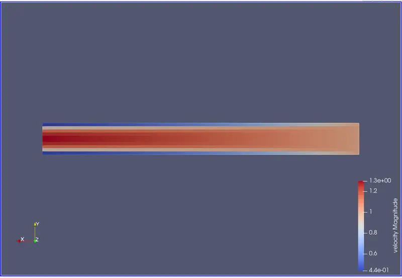
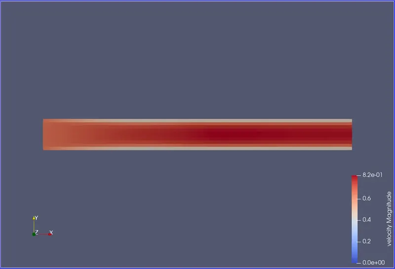
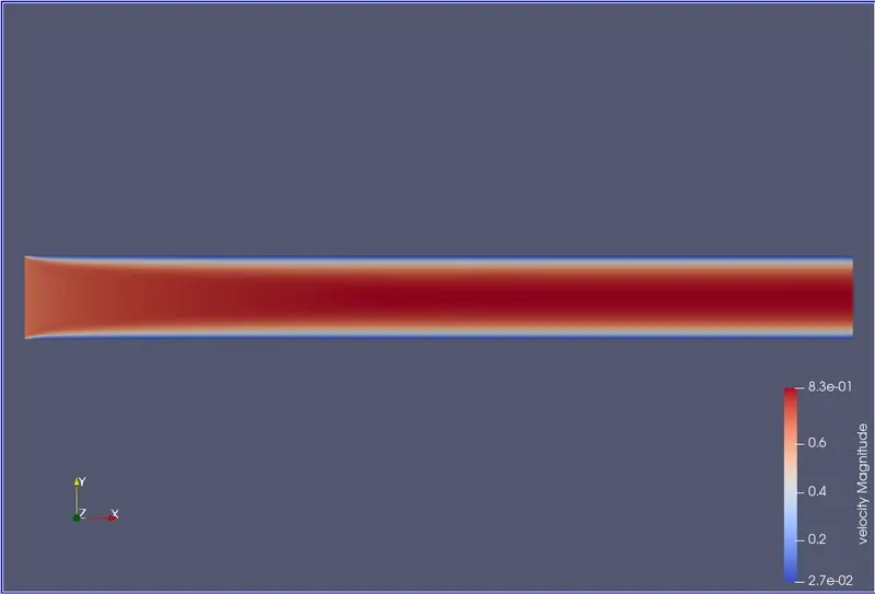
- Velocity contour
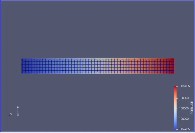
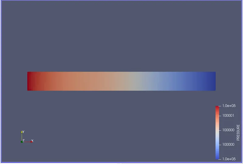
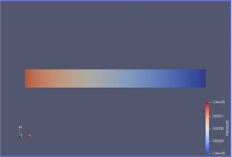
- Pressure Contour
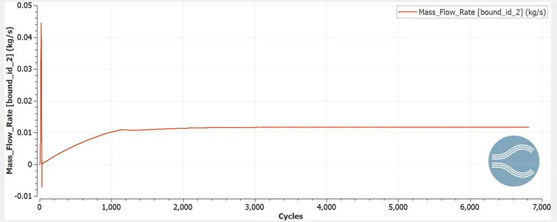
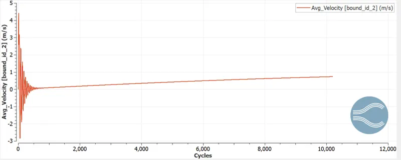
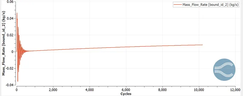
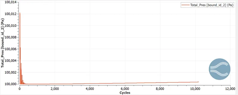
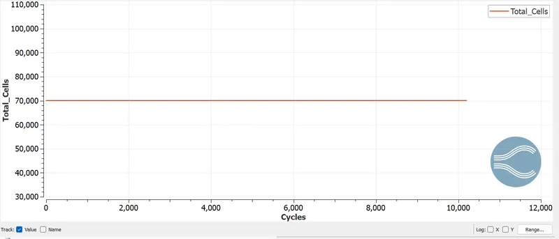
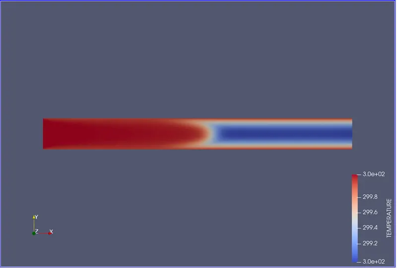
- Plots
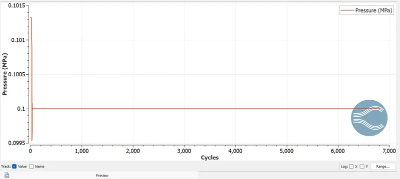
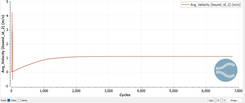
- Grid Size
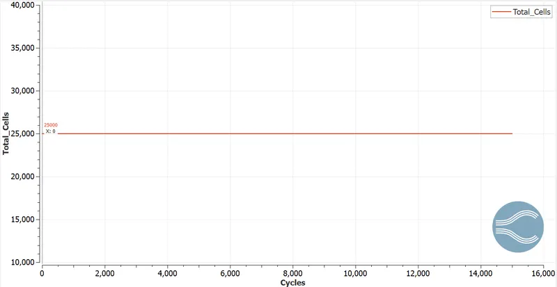
- dx = 2e-4m, dy = 2e-4m, dz = 2e-4m
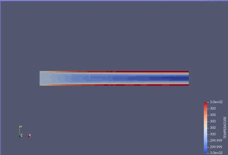
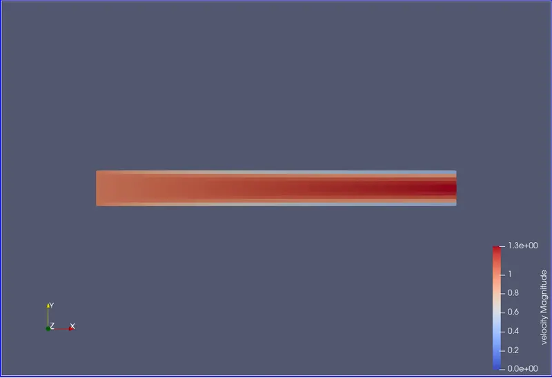
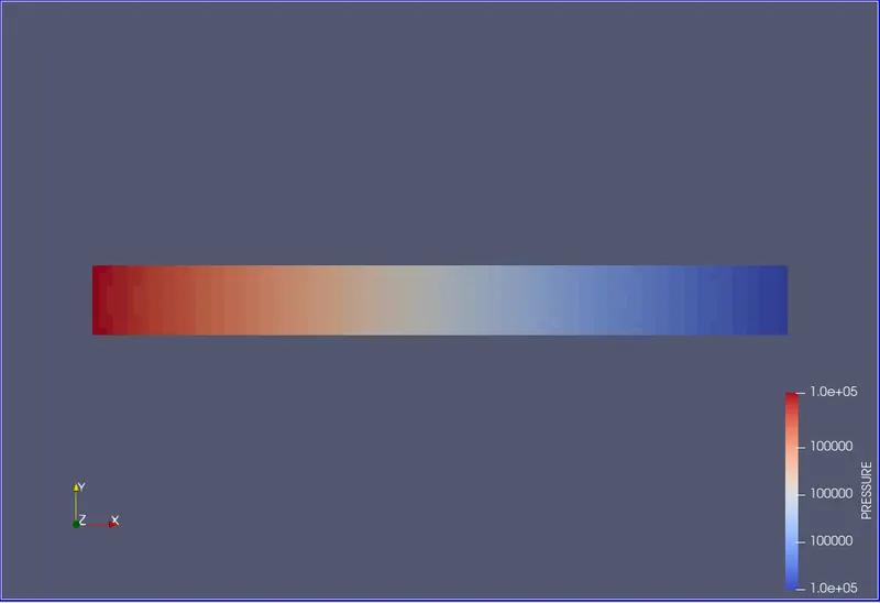
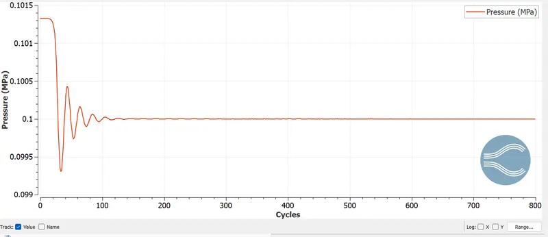
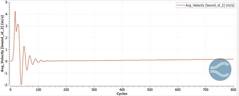
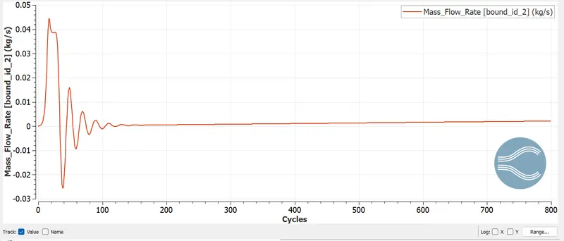
- Grid Size
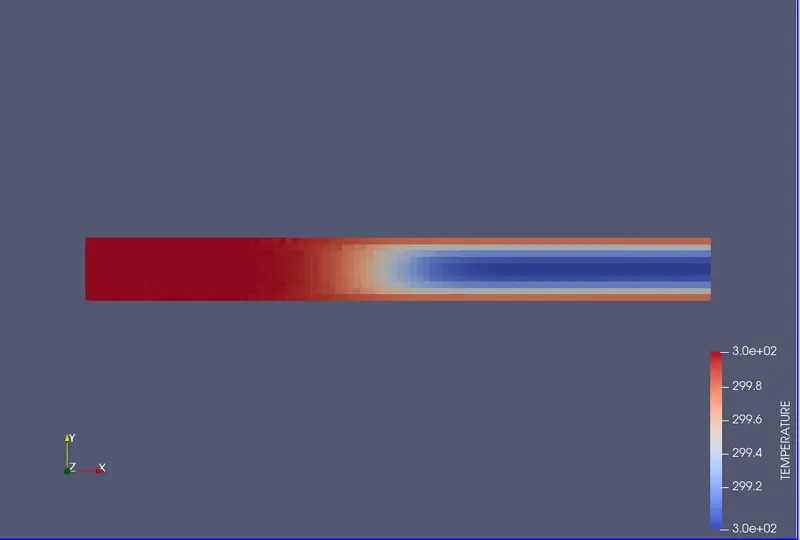
- dx = 1.5e-4m, dy = 1.5e-4m, dz = 1.5e-4m
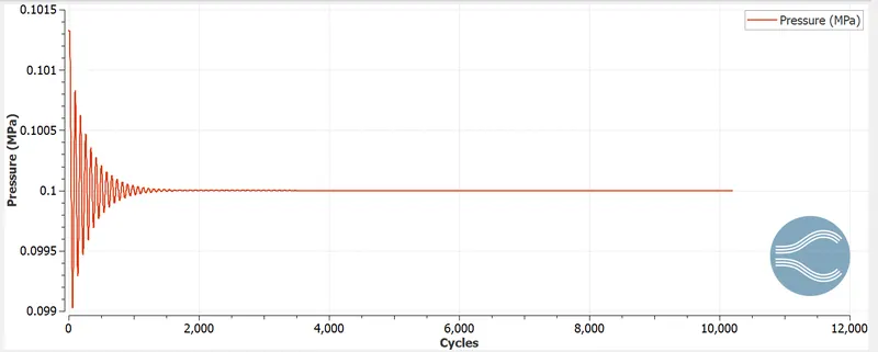
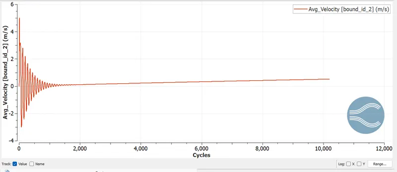
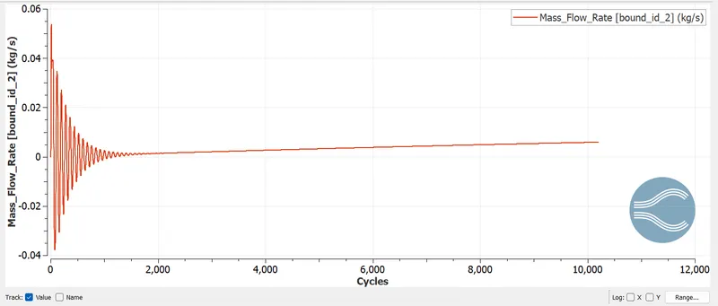
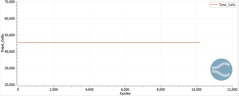
- Grid Size
- dx = 1.0e-4m, dy = 1.0e-4m, dz = 1.0e-4m (If this is too much for your PC, use 1.2e-4m)
- 1.2e-4m
- Google drive link for animation.
- https://drive.google.com/drive/folders/12fs33LKrGpqQRg0brV7P8WP-QjQkutFw
- Stepwise Explaination
- Create the duct flow geometry at the convergence using the Create option.
- Defines the boundaries to each surface of the geometry.
- Specify the normal direction inside the face.
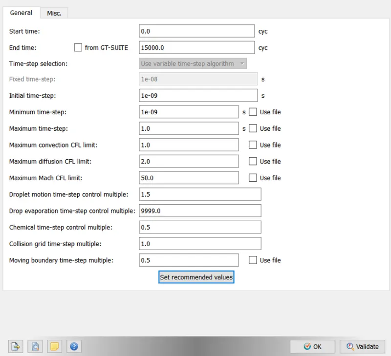
- The setup defines materials, simulation parameters, fluid domains, boundary conditions, number of cycles and grid definition.
- Extract the setup files in the simulation folder.
- The Transform panel was used because by default normals point outwards from the geometry. Select any plane and press Apply to change the normal direction.
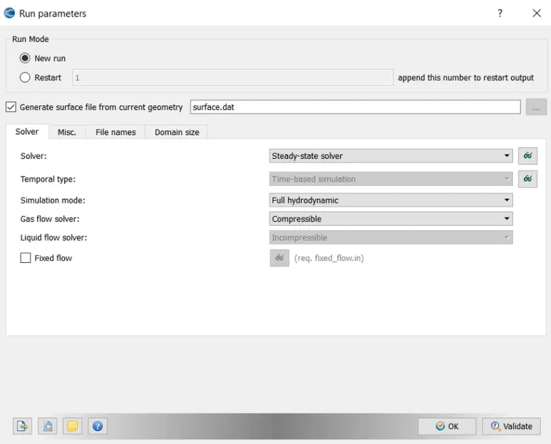
- To run normal steady-state simulations in the setup application type, the time-based option should be selected. The run parameter defines the solver as a stationary solver is set.
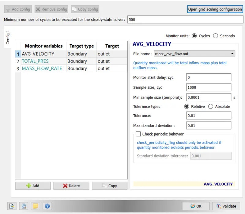
- In other sections, we turned on the steady-state monitor to monitor the steady-state speed of cycle convergence.
- A speed monitor is set with the correct tolerance to track the speed at which results converge.
- Run the entire Cygwin setup file.
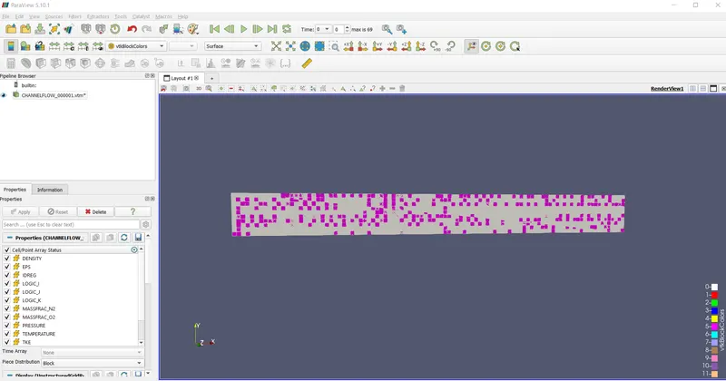
- Post-process all results and open in Paraview. Display the mesh for all three mesh bases.
- Draws velocity and pressure contours for all three basic mesh sizes.
- Plots of velocity, pressure, mass flow rate, and total cell number for all three basic mesh sizes.
- Create an animation in Paraview to show the unfolding of the flow.
- Describe the plot and write a detailed report on the project.
- Observation
- We observe that the first case has the highest speed, but is generally not preferred to be exact due to the coarser mesh.
- Two cases are calculated more precisely.
- The mass flow rate at the outlet of the purified casing is approximately the same. Positive and negative flows can be observed when comparing both inlet and outlet.
- The finer the mesh, the clearer the velocity profile obtained compared to his other two cases.
- Therefore, the larger the size, the clearer and more accurate the results obtained.
- As networks become finer and finer, the total number of cells increases, and computation time increases as the number of cells increases.
- Mass flow rate is directly proportional to density and velocity. So, by increasing mass flow rate velocity increases.
- Conclusion:
- Converge CFD hydrographic simulation is performed. Different mesh sizes give accurate results.
- A low grid resolution simulation will simulate the result in the least amount of time, but the result will be slightly less accurate and smoother. Therefore, it is recommended to run the first simulation with a coarse mesh to get an overview of the simulation.
- Fine Mesh Simulation is recommended to be used for final simulation with the same proven settings.
- Simulating the results with different grid sizes is very important to validate the mesh independence test.
- Velocity is higher in the center and lower near the walls due to wall shear stress.