Week 3.5 - Deriving 4th order approximation of a 2nd order derivative using Taylor Table method

• Derive the following 4th order approximations of the second-order derivative.

  1. Central difference

  2. Skewed right-sided difference

  3. Skewed left-sided difference

• Objective - To derive the 4th order approximations of the second-order derivative using taylor table method for Central difference, Skewed right-sided difference, Skewed left-sided difference and write a program in Matlab to evaluate the second-order derivative of the analytical function exp(x)*cos(x) and compare it with the 3 numerical approximations that you have derived.
• A Taylor series can be used to calculate the value of an entire function at each point if the value of the function and all its derivatives is known at a single point.
• Formulation for taylor table method :

• f′′(x) = af(x−2h) + bf(x−h) + cf(x) + df(x+h) + e(x+2h) /h^2

  Formulation for the Taylor table method of left Skewed schme

  f′′(x) = af(x) + bf(x−h) + cf(x−2h) + df(x−3h) + ef(x−4h) + ff(x−5h) /h^2

  Formulation for the Taylor table method of Right-Skewed schme

  f′′(x) = af(x) + bf(x+h) + cf(x) + bf(x+h) + cf(x+2h) + df(x+3h) + ef(x+4h) + ff(x+5h) /h^2

  Forward difference schme

  f′′(x) = af(x) + bf(x+h) + cf(x+2h) /h^2

  Backward difference schme

  f′′(x) = af(x) + bf(x−h) + cf(x−2h) /h^2

• Scheme derivations :
• Central differencing Scheme-
• formula- No. of nodes = p +q -1

where, p is order of derivative

q is order of approximations

No. of nodes = 2 +4 -1 = 5

code- For central differencing scheme.Input values taken from derivation.

close all
clear all
clc

%input for matrix A
A = [1 1 1 1 1;-2 -1 0 1 2;2 1/2 0 1/2 2;-4/3 -1/6 0 1/6 4/3;2/3 1/24 0 1/24 2/3]

%input for matrix B
B = [0;0;1;0;0]

%Linsolve
X = linsolve(A,B)

• Derivation : Hypothesis Equation -

(△x^2)(δ^2f /δx^2) = a⋅f(i−2) + b⋅f(i−1) + c⋅f(i) + d⋅f(i+1) + e⋅f(i+2)

△x^n⋅f^n(i)	△x⋅f′(x)	△x⋅f'(x)	△x^2⋅f''(x)	△x^3⋅f'''(x)	△x^4⋅f^iv(x)	△x^5⋅f^v(x)	△x^6⋅f^vi(x)
a⋅f(i−2)	a	−2a	2a	−4a/3	2a/3	−4a/15	4a /45
b⋅f(i−1)	b	−b	b /2	−b /6	b /24	−b1 /20	b /720
c⋅f(i)	c	0	0	0	0	0	0
d⋅f(i+1)	d	d	d /2	d /6	d/24	d /120	d /720
e⋅f(i+2)	e	2e	2e	4e/3	2e/3	4e /15	4e/45
(△x^2)(δ^2f /δx^2)	0	0	(δ^2f /δx^2)	0	0	-

Equations-

a + b + c + d + e =0

−2a −b + d + 2e =0

2a + b/2 + d/2 + 2e =1

−4a/3 − b/6 + d/6 + 4e/3 =0

2a /3 + b /24 + d /24 + 2e /3 =0

Output -

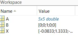
A =

1 1 1 1 1
-2 -1 0 1 2
2 1/2 0 1/2 2
-4/3 -1/6 0 1/6 4/3
2/3 1/24 0 1/24 2/3

B =

0
0
1
0
0

X =

-1/12
4/3
-5/2
4/3
-1/12

>>

• Skewed Right sided difference
• No. of nodes = p + q

where, p is order of derivative.

q is order of approximation.

No. of nodes = 2+4 =6

• Code for Skewed right sided difference

Input values taken from derivation.

close all
clear all
clc

format rational
%input for matrix A
A = [1 1 1 1 1 1;
     0 1 2 3 4 5;
     0 1/2 2 9/2 8 25/2;
     0 1/6 8/6 27/6 64/6 125/6;
     0 1/24 16/24 81/24 256/24 625/24;
     0 1/120 32/120 243/120 1024/120 3125/120]
%input for matrix B
B = [0;0;1;0;0;0]

%Linsolve
X = linsolve(A,B)

Hypothesis equation -

(△x^2)(δ^2f /δx^2) = a⋅f(i) + b⋅f(i+1) + c⋅f(i+2) + d⋅f(i+3) + e⋅f(i+4) + g⋅f(i+5)

Taylor table-

△x^n⋅f^n(i)	△x⋅f′(x)	△x⋅f'(x)	△x^2⋅f''(x)	△x^3⋅f'''(x)	△x^4⋅f^iv(x)	△x^5⋅f^v(x)
a⋅f(i)	a	0	0	0	0	0
b⋅f(i+1)	b	b	b/2	b/6	b/24	b/120
c⋅f(i+2)	c	2c	4c/2	8c/6	16c/24	32c/120
d⋅f(i+3)	d	3d	9d/2	27d/6	81d/24	243d/120
e⋅f(i+4)	e	4e	16e/2	64e/6	256e/24	1024e/120
g⋅f(i+5)	g	5g	25g/2	125g/6	625g/24	3125g/120

Equations-

a + b + c + d + e + g = 0

0 + b + 2c + 3d + 4e + 5g = 0

0 + b /2 + 4c/2 + 9d /2 + 16e/2 + 25g/2 = 1

0 + b/6 + 8c/6 + 27d/6 + 64e/6 + 125g/6 = 0

0 + b/24 + 16c/24 + 81d/24 + 256e/24 + 625g/24 = 0

0 + b/120 + 32c/120+ 243d/120 + 1024e/120 + 3125g/120 = 0

Output -

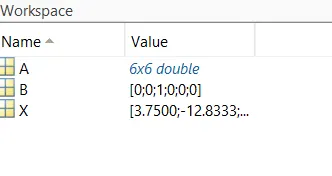
A =

1 1 1 1 1 1
0 1 2 3 4 5
0 1/2 2 9/2 8 25/2
0 1/6 4/3 9/2 32/3 125/6
0 1/24 2/3 27/8 32/3 625/24
0 1/120 4/15 81/40 128/15 625/24

B =

0
0
1
0
0
0

X =

15/4
-77/6
107/6
-13
61/12
-5/6

>>

• Skewed left-sided difference-

No. of nodes = p + q

where, p is order of derivative.

q is order of approximation.

No. of nodes = 2+4 =6

• Code for Skewed left sided difference

Input values taken from derivation

close all
clear all
clc

format rational
% A = [1 1 1 1 1;-2 -1 0 1 2;2 1/2 0 1/2 2;-4/3 -1/6 0 1/6 4/3;2/3 1/24 0 1/24 2/3]
% B = [0;0;1;0;0]
% X = linsolve(A,B)

%input for matrix A
A = [1 1 1 1 1 1;
     0 -1 -2 -3 -4 -5;
     0 1/2 2 9/2 8 25/2;
     0 -1/6 -8/6 -27/6 -64/6 -125/6;
     0 1/24 16/24 81/24 256/24 625/24;
     0 -1/120 -32/120 -243/120 -1024/120 -3125/120]

%input for matrix B
B = [0;0;1;0;0;0]

%Linsolve
X = linsolve(A,B)

Hypothesis eqn - (△x^2)(δ^2fδx^2) = a⋅f(i) + b⋅f(i−1) + c⋅f(i−2) + d⋅f(i−3) + e⋅f(i−4) + g⋅f(i−5)

• Taylor table -

• △x^n⋅f^n(i)	f(i)	△x⋅f′(x)	△x^2⋅f′′(x)	△x^3⋅f′′′(x)	△x^4⋅f^iv(x)	△x^5⋅f^v(x)
  a⋅f(i)	a	0	0	0	0	0
  b⋅f(i-1)	b	-b	b/2	-b/6	b/24	-b/120
  c⋅f(i-2)	c	-2c	4c/2	8c/6	16c/24	-32c/120
  d⋅f(i-3)	d	-3d	9d/2	-27d/6	81d/24	-243d/120
  e⋅f(i-4)	e	-4e	16e/2	-64e/6	256e/24	-1024e/120
  g⋅f(i-5)	g	-5g	25g/2	−125g/6	625g/24	-3125g/120
  (△x^2)(δ^2fδx^2)	0	0	(δ^2f /δx^2))	0	0	0

Equations-

a + b + c + d + e + g = 0

0 - b -2c -3d - 4e - 5g = 0

0 + b /2 + 4c/2 + 9d/2 + 16e/2 + 25g/2 = 1

0 - b/6 - 8c/6 - 27d/6 - 64e/6 - 125g /6 =0

0 + b /24 + 16c/24 + 81d/24 + 256e/24 + 625g /24 = 0

0 − b/ 120 − 32c /120 − 243d / 120 − 1024e / 120 − 3125g /120 = 0

Output-

A =

1 1 1 1 1 1
0 -1 -2 -3 -4 -5
0 1/2 2 9/2 8 25/2
0 -1/6 -4/3 -9/2 -32/3 -125/6
0 1/24 2/3 27/8 32/3 625/24
0 -1/120 -4/15 -81/40 -128/15 -625/24

B =

0
0
1
0
0
0

X =

15/4
-77/6
107/6
-13
61/12
-5/6

>>

• Main code -

• clear all
  close all
  clc
  
  %given the value of x
  x =pi/3 ; 
  
  %declaring the range for the dx
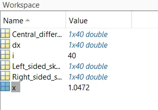
  dx = linspace(pi/4000,pi/40,40);
  
   for i =1:length(dx)
  
      Central_differencing(i) = fourth_order_central_differencing(x,dx(i));
      Right_sided_skew(i) = fourth_order_right_sided_skew(x,dx(i));
      Left_sided_skew(i) = fourth_order_left_sided_skew(x,dx(i));
  
   end
  
   %graph plotting
   loglog(dx, Central_differencing,'g','Linewidth',3)
   hold on
   loglog(dx,Right_sided_skew,'r','LineWidth',3)
   hold on
   loglog(dx,Left_sided_skew,'b','LineWidth',3)
  
   legend('Central differencing','Skewed right sided difference','Skewed Left sided difference')
   xlabel('Range of dx')
   ylabel('Truncation Error')
  

• Results-

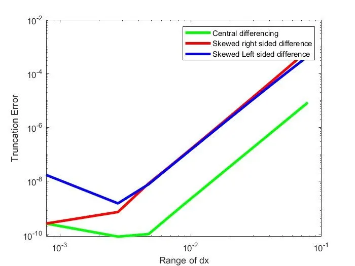
Truncation error vs Range of dx

• Stepwise Explaination of code -
• To calculate the first order, second order, and fourth-order approximations, functions of each order are created and called in the main function.
• After defining the functions for first order, second order and fourth order approximations ,we can proceed for the main program for range of dx.
• For each function analytical and numerical derivates are calculated.
• Then we have to calculate analytical derivative for the given function at x = pi/3.
• Declaring the range for dx, i.e, dx range = [pi/4000,pi/40]
• Then to compute the approximations for varying dx value, linspace command is used and declared the 40 values.
• For loop command is used for definining the function errors.
• First order error,Second order error and fourth order error are calculated.
• After the error values are obtained ,the loglog plot command is used to plot the graph.
• Here ,we 'dx' vs 'error' graph are plotted.
• Linewidth is given for first order , second order and fourth order approximation.

• Conclusion-
• We can see that the error is more for skewed schemes than for the central differencing schemes.
• For small dx values round up errors would be high.
• Central differencing scheme is better than other schemes beacuse is gives accurate and approximate values.
• Since ,the left-right skewed difference method uses data from only one side of the point of interest, it provides less approximate and accurate values ​​about the point.

• why a skewed scheme is useful?

A system that does not contain sufficient information on either side of the point of interest. In such cases, we cannot use the central difference scheme, so the skew scheme is useful in such cases.

• What can a skewed scheme do that a CD scheme cannot?

CDS cannot be used on border nodes due to unavailability of right and left nodes at the same time. In such cases,the skewed difference scheme is used.