Week 4.1 - Solving second order ODEs

• Write the code for the given ODE which represents the equation of motion of a simple pendulum with damping
• Objective- To write a program that solves the following ODE. This ODE represents the equation of motion of a simple pendulum with damping. Simulate the pendulum motion between 0-20 sec, for angular displacement=0,angular velocity=3 rad/sec at time t=0.

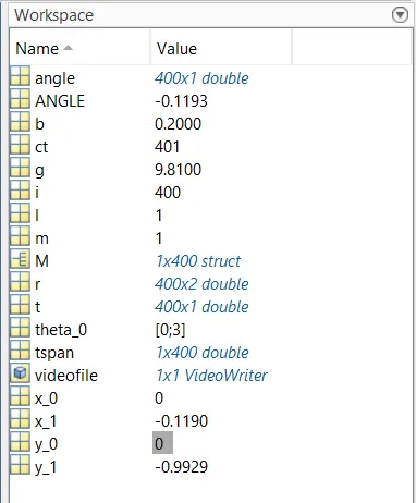
• clear all
  close all
  clc
  
  %state variables definition
  l=1 ;
  m=1 ;
  b=0.2 ;
  g=9.81 ;
  
  %Initial condition angular displacement and angular velocity
  theta_0=[0;3];
  tspan=linspace(0,20,400);
  
  %solving the ODE
  [t,r]=ode45(@(t,theta) ode_funct(t,theta,b,g,l,m),tspan,theta_0);
  figure(1)
  plot(t,r(:,1),DisplayName='Angular displacement')
  hold on
  plot(t,r(:,2),DisplayName='Angular velocity')
  legend
  xlabel('plot')
  ylabel('time')
  
  %Animation of pendulum
  ct=1;
  angle=[r(:,1)];
  for i=1:length(angle)
      ANGLE = angle(i)
      x_0=0;
      y_0=0;
      x_1=1*sin(ANGLE);
      y_1=-1*cos(ANGLE);
  
   figure(2)
      plot([x_0 x_1],[y_0 y_1],'linewidth',1,'Color','b')
      hold on 
      plot(x_1,y_1,'o','MarkerSize',6,'Color','r')
      axis([-3 3 -3 3])
      pause(0.001)
      hold on
      plot([-2 2],[0 0])
      M(ct)=getframe(gcf);
      hold off
      ct=ct+1;
  end
  movie(M)
  videofile =VideoWriter('simple_pendulum12.avi','Uncompressed AVI');
  open(videofile)
  writeVideo(videofile,M)
  close(videofile)
  
  
  
  
  
  
  
  ​

  • Step by step coding explaination-
  • Code started with the ‘%’ command.
  • Then assign the values as per the given data.
  • After assigning the data, ‘ode45()’ command is given to solve the above equation.
  • Among the ode solvers, ode45 is usually the function of choice used to estimate the error and determine step size.
  • The ‘ode45’ command is used to integrate system of differential equations from initial to final conditions.
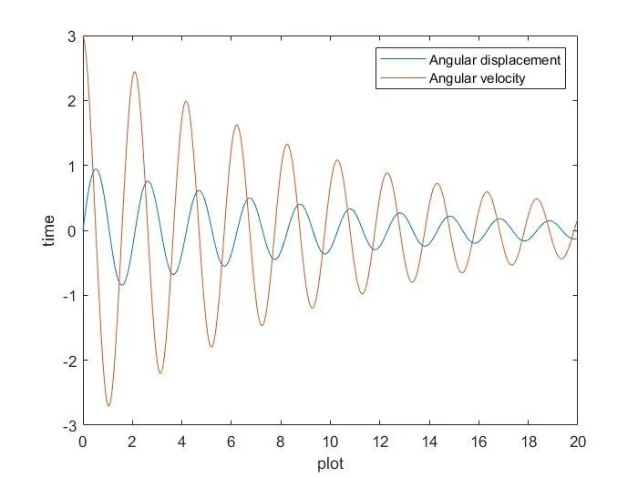
  • Then values are plotted as per the given code to get the above result.
  • So in this way,the above ode’s equation gets solved using matlab.
  • Ode45 works only with functions that use two input arguments, t and r as given in the code.
  • Plot command is given to get the graph.
  • Time vs velocity graph are plotted .

• Results-

‘ODE45’ SYNTAX:

• Syntax for ode45 can be given as,

Ode45(ode_function(),t_span,y0)

Where, t_span and y0 are limits for integration.

• Ode45 are automatic stepsize Runge kutta Fehlberg intergration method used to integrate the system of differential equations of second order differential equation.

Explaination-

• Code started with the ‘%’ command.
• Then assign the values as per the given data,i,e state variables are defined. Initial conditions are given for angular displacement and angular velocity.
• Linspace command is used to create an evenly spaced sequence in a specified interval.
• For loop command is used for assigning the different values to theta.
• Plot command are given to plot the graph. xlabel(velocity) vs ylabel(time) graph are plotted.
• For animation,ct =1, ct =ct+1 command are given
• For making animation video,used

movie(M)

videofile =VideoWriter('simple_pendulum1.avi','Uncompressed AVI');

open(videofile)

writeVideo(videofile,M)

close(videofile)

Here,the above code executes for creating the video file.

• So,this was the explaination for the above code for animating the simple pendulum.

You tube link-

https://youtu.be/gTKe8Bd9CHo