Week 1: Channel flow simulation using CONVERGE CFD
INTRODUCTION:
Channel flow is an internal flow in which the confining walls change the hydrodynamic structure of the flow from an arbitrary state at the channel inlet to a certain state at the outlet. The simplest illustration of internal flow is a laminar flow in a circular tube, while a turbulent flow in the rotor of a centrifugal compressor is an example of the most intricately shaped internal flow. Engineering devices employ channels with cross-sections of various geometrical shapes.
In this project, Converge Studio was used to establish a working idea of airflow simulation through a channel flow under certain parameters, which will be elaborated systematically in this report.
OBJECTIVE:
- Setup channel flow simulation.
- Run simulation for 3 different mesh sizes.
- Plot velocity and pressure contours for 3 different mesh sizes.
- Show plots for velocity, pressure, mass flow rate, and total cell count for all 3 mesh sizes.
PROCEDURE:
GEOMETRY
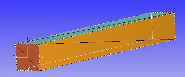
- Creating a geometry using the creation tool of Converge Studio.
- Running diagnosis to check if there are any open edges or faces.
- Checking the orientation of Normals, The normal should be such that their orientation is pointing towards the fluid flow.
BOUNDARY FLAGGING
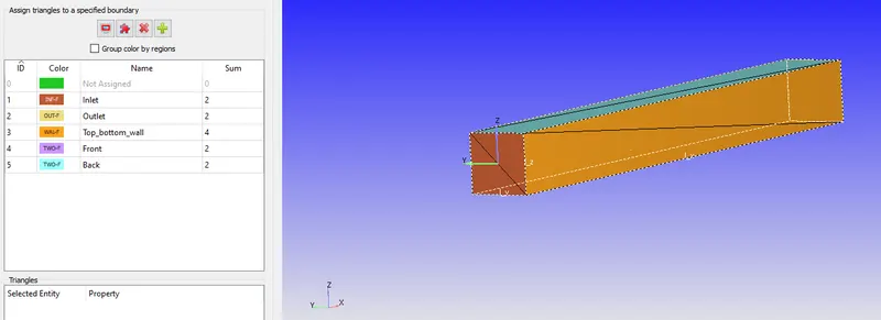
The boundaries are flagged. The converge studio basically uses triangular blocks to create geometry. So by selecting the triangles boundaries are Flagged
- Inlet
- Outlet
- Top and Bottom Walls
- Front2D
- Back2D
CASE SETUP:
Application type: Time based
Materials: Predefines mixture: Air
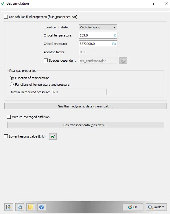
Gas Simulation:
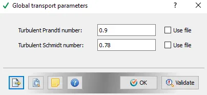
Global Transport Parameters:
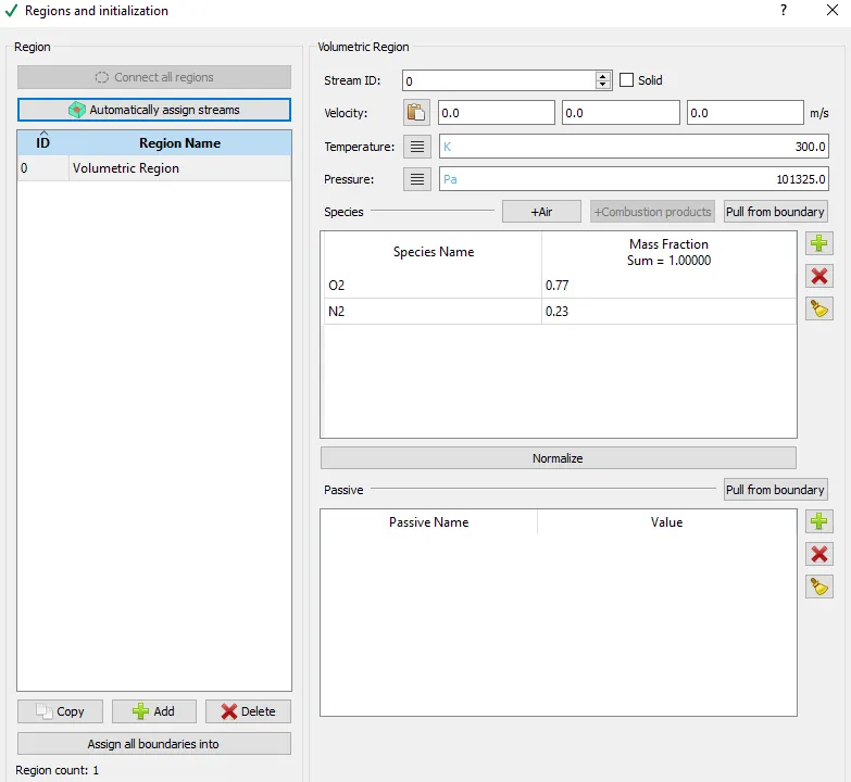
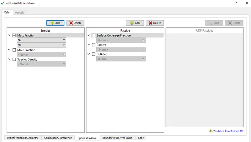
Species: N2 and O2 are added to the list.

SIMULATION PARAMETERS:
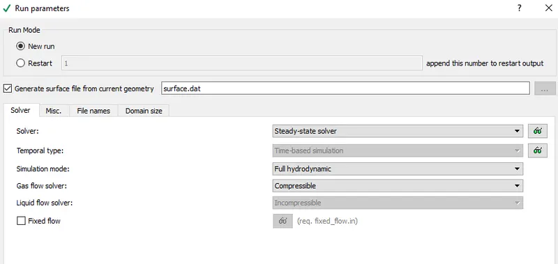
Run Parameters:
Steady state solver has been taken.
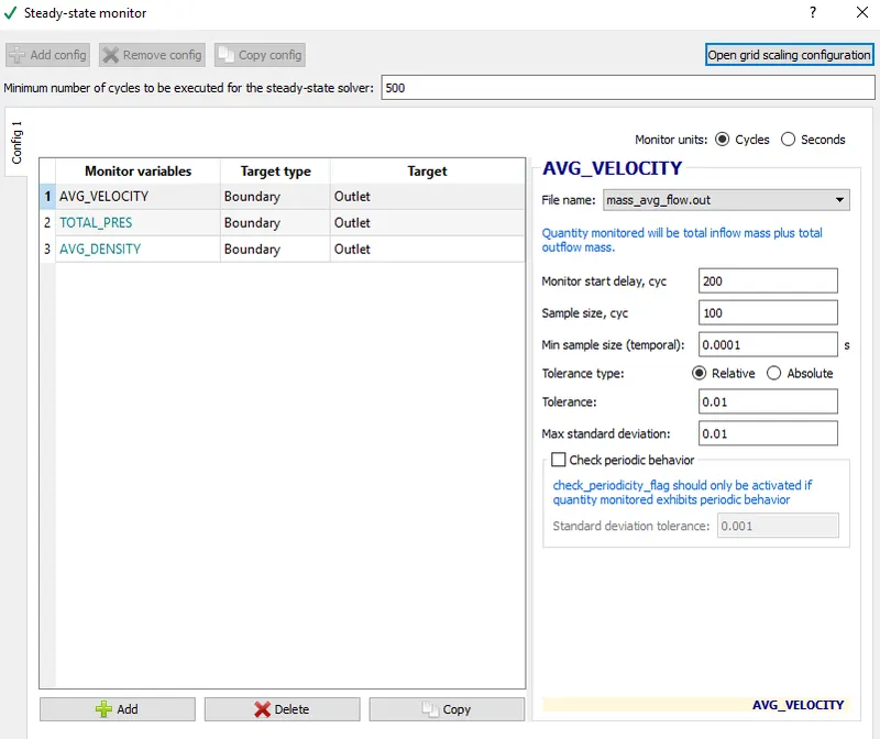
Steady state Monitor:
Average velocity, total pressure and average density are the monitor variables enabled.
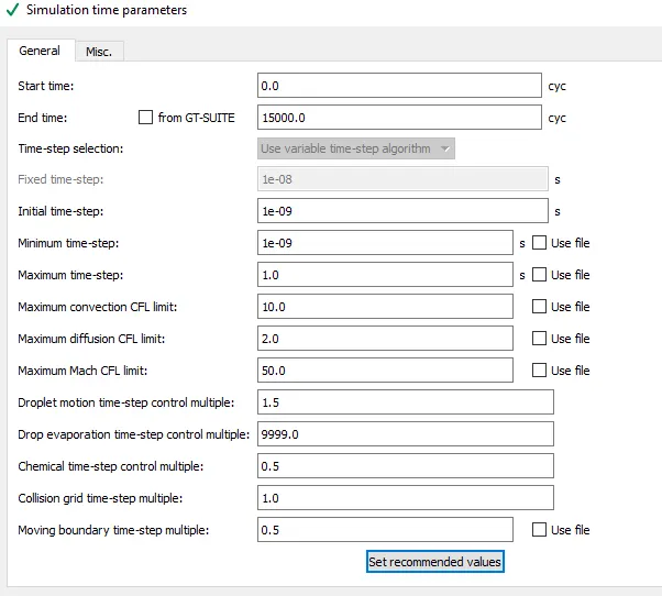
Simulation time Parameters:
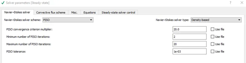
Solver parameters:
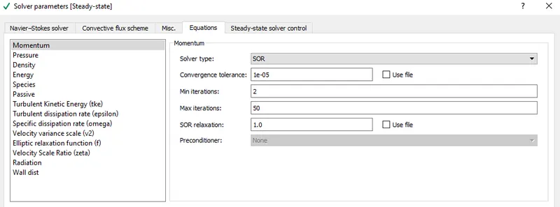
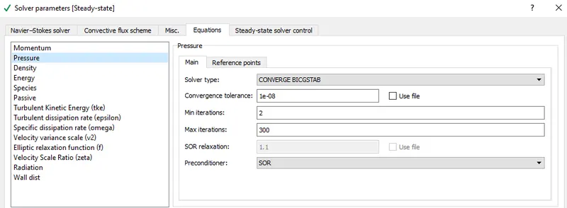
BOUNDARY CONDITIONS:
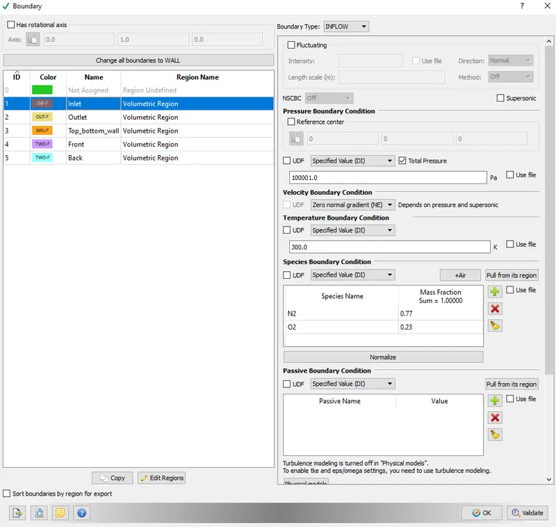
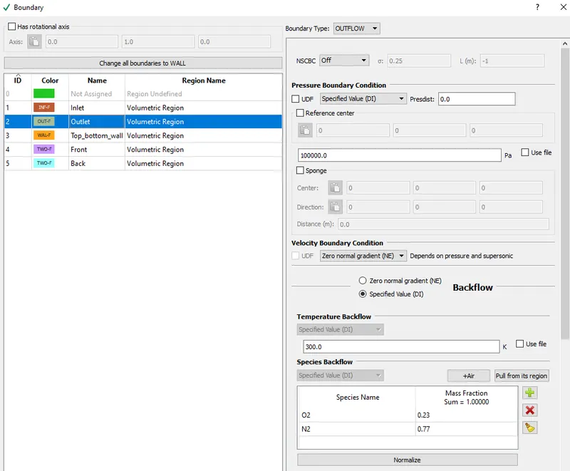
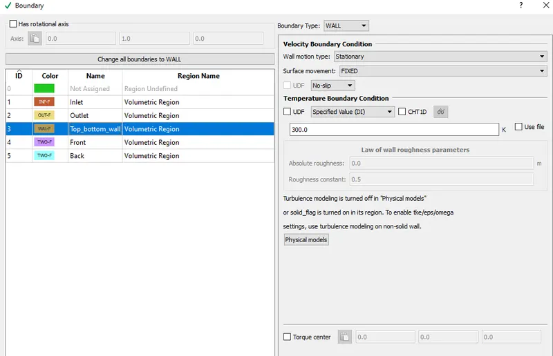
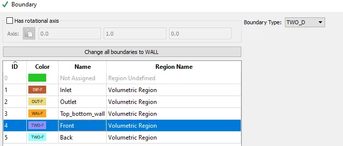
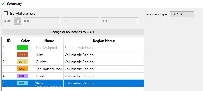
Regions & Initialisation:
Physical Models:
Turbulence modelling has been disabled.
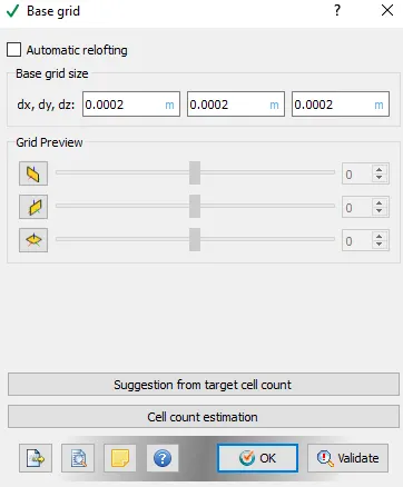
Grid size:
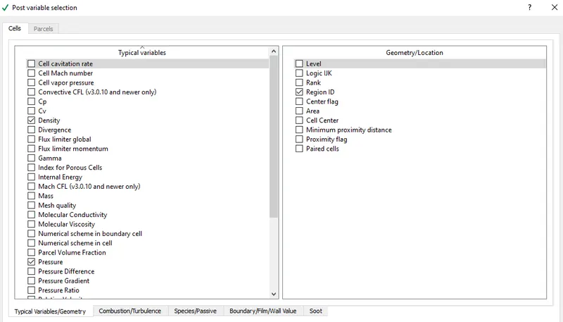
Post variable selection:
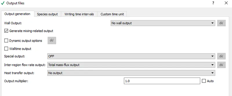
Output files:
- Once the case setup is complete all the input files are exported to a specific folder
- Then Cygwin is used to solve the inputs and once the simulation is complete converge converts the result data into a format that can be read by Paraview.
- Post-processing is done in Paraview.
Resuts
Case-1
Grid size:- dx = 2e-4m, dy = 2e-4m, dz = 2e-4m
Mesh:

Velocity contour:
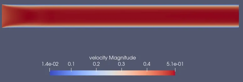
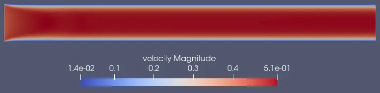
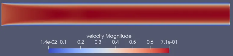
From the above plot we can say that velocity is high at the centre and keeps on decreasing and lower near the walls.
PRESSURE CONTOUR:
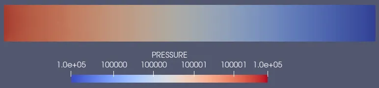
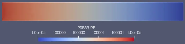
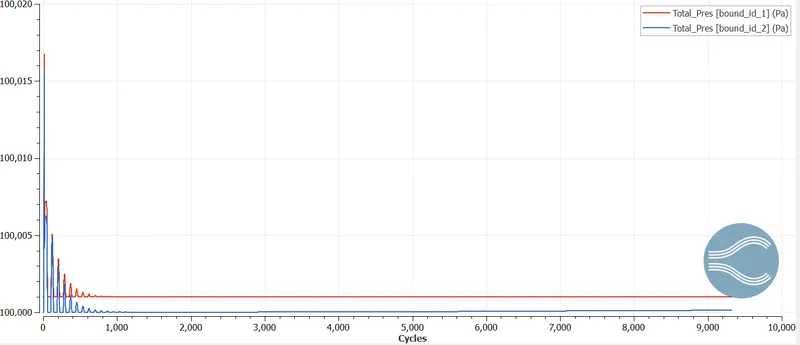
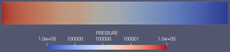
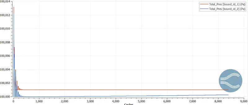
From the above plot, the pressure is higher at inlet and lower at outlet. Due to this pressure difference the flow takes place in the channel.
Mass flow rate plots:
Velocity Plots:
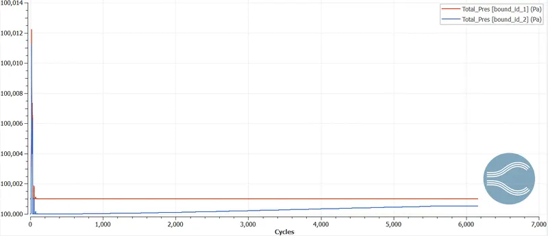
Pressure Plots:
Case-2
Grid size:- dx = 1.5e-4m, dy = 1.5e-4m, dz = 1.5e-4m
Mesh:

Velocity contour:
PRESSURE CONTOUR:
Mass flow rate plots:
Velocity Plots:
Pressure Plots:
Case-3
Grid size:- dx = 1.0e-4m, dy = 1.0e-4m, dz = 1.0e-4m
Mesh:

Velocity contour:
PRESSURE CONTOUR:
Mass flow rate plots:
Velocity Plots:
Pressure Plots:
Observations:
- From the simulation performed it is clear that for mesh size(2e-4, 1.5e-4, 1.0e-4) the total cell count for each of the mesh is 25000, 45000, 100000 respectively. Hence as the mesh becomes finer and finer the total cell count increases, as the cell count increases the computational time also increases.
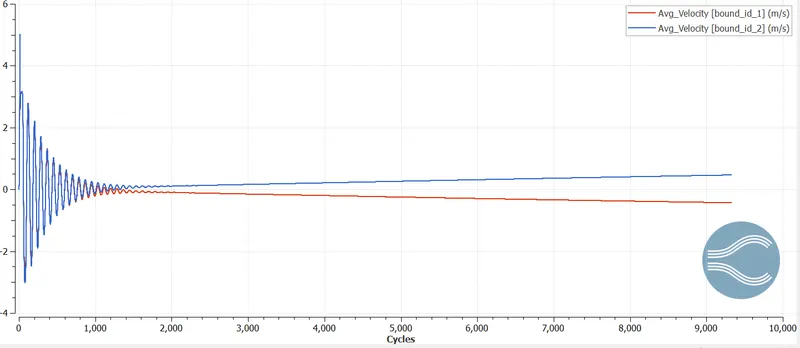
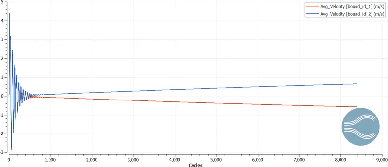
- It is observed that velocity in the initial case is highest but as the mesh is coarse it is generally not preferred to be accurate. In nest two cases it is calculated more accurately.
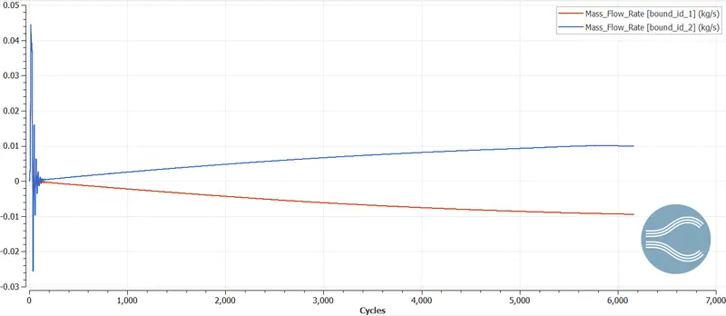
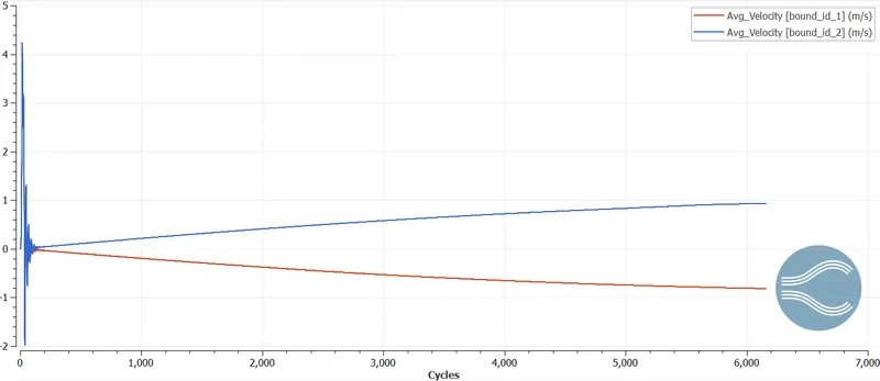
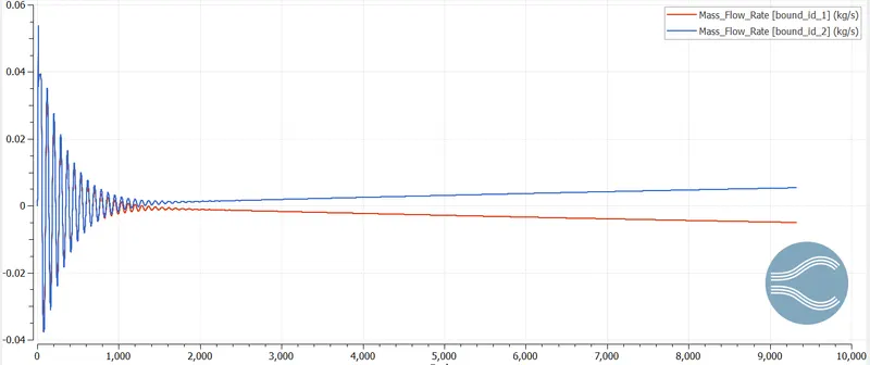
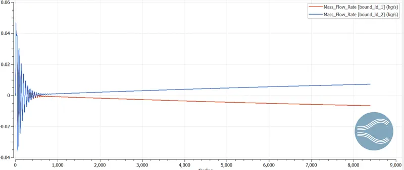
- The mass Flow Rate at the outlets for the refined cases is almost the same. When both inlets and outlets are compared we can observe a positive and a negative flow.
- As the mesh becomes finer, the velocity profile obtained is also much clear compared to the other 2 cases.
- Hence, as the size increases the results obtained are much clear and accurate
Vl. CONCLUSION:
The channel flow simulation using Converge CFD is performed. With different mesh sizes, accurate results are obtained.