Week 3 - Solving second order ODEs

AIM

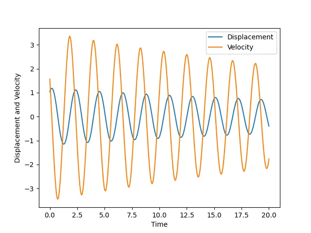
• Write a program in Python that will simulate the pendulum motion by solving the given 2nd order ODE and plot a graph showing dispacement and velocity vs time.

THEORY

In Engineering, ODE is used to describe the transient behavior of a system. A simple example is a pendulum

The way the pendulum moves depends on the Newtons second law. When this law is written down, we get a second order Ordinary Differential Equation that describes the position of the "ball" w.r.t time.

The second order ODE for simple pendulum is given as,

`(del^2theta)/(delt)+(b/m)(deltheta)/(delt)+(g/L)sintheta=0`

Where,

b=damping coefficient

m=mass of the ball in kg

g=acceleration due to gravity in `m/s^2`

L=Length of the pendulum in m

Inputs,

b=0.05

m=1 kg

g=9.81 `m/s^2`

L=1 m

SOLVING METHOD

To solve a higher order ODE analytically/numerically we have to break them into first order ODEs. Since this is a 2nd order ODE we need to break them into two first order ODEs,

Let,

`theta=theta_1`

So, `(deltheta)/(delt)=(deltheta_1)/(delt)`

Let's assume,

`(deltheta_1)/(delt)=theta_2`..................eqn(1)

Put the above equation in the simple pendulum equation,

Then we get,

`(deltheta_2)/(delt)+(b/m)theta_2+(g/L)sintheta_1=0`

Rearranging,

`(deltheta_2)/(delt)=-(b/m)theta_2-(g/L)sintheta_1`..................eqn(2)

Finally we got two first order ODEs(eqn(1)&(2))

To solve in program, we have to make the equations into matrix form.

`del/(delt)[[theta_1],[theta_2]]=[[theta_2],[-(b/m)theta_2-(g/L)sintheta_1]]`

This is called as solution vector.

Since we are solving two 1st order ODEs we need two initial conditions.

• The first one represents angular dispacement`(theta_2)`
• The second one represents angular velocity`((deltheta_2)/(delt))`

PYTHON CODE

import math
import matplotlib.pyplot as plt
import numpy as np
from scipy.integrate import odeint


def model(theta,t,b,g,l,m):
	theta1=theta[0]
	theta2=theta[1]
	dtheta1_dt=theta2
	dtheta2_dt=-(b/m)*theta2-(g/l)*math.sin(theta1)
	dtheta_dt=[dtheta1_dt,dtheta2_dt]
	return dtheta_dt

# inputs
b=0.05
g=9.81
l=1
m=1

# initial condition
theta_0=[math.pi/3,math.pi/2]

# time points
t=np.linspace(0,20,300)

# solving ode
theta=odeint(model,theta_0,t,args=(b,g,l,m))


#plotting
plt.plot(t,theta[:,0],label='Displacement')
plt.plot(t,theta[:,1],label='Velocity')
plt.legend()
plt.xlabel('Time')
plt.ylabel('Displacement and Velocity')
plt.show()

# animation

y=theta[:,0]



ct=1
for angle in y:
	x1=0
	y1=2
	x2=-l*math.sin(angle)
	y2=-l*math.cos(angle)

	filename = '%05d.png' %ct
	ct=ct+1

	plt.figure()
	plt.plot([x1,x2],[y1,y2],linewidth=2)
	plt.plot(x2,y2,'o','marker',markersize=20,color='k')
	plt.plot([-1.5,1.5],[2,2],linewidth=5)
	plt.xlim([-2.5,2.5])
	plt.ylim([-2.5,2.5])
	plt.title('Pendulum animation')
	plt.savefig(filename)

• CODE FOR ANIMATION

For animation we need to use the command prompt.

C:\Users\Skill_Lync\Desktop\Gok\1\10.pendulum>cd C:\Users\Skill_Lync\Desktop\Gok\1\10.pendulum

C:\Users\Skill_Lync\Desktop\Gok\1\10.pendulum>magick *.png pendulum.gif

EXPLANATION OF CODES

• import math - This command is used to import math module, which extends the list of mathematical functions. To use it, we must import the math module.
• import matplotlib.pyplot as plt - This command is used to import matplotlib.pyplot, which is a collection of functions that make matplotlib work like MATLAB. Each pyplot function makes some change to a figure: e.g., creates a figure, creates a plotting area in a figure, plots some lines in a plotting area, decorates the plot with labels, etc. We simply assigned matplotlib.pyplot to plt for easiness.
• import numpy as np - It is used to import NumPy, which is a Python library used for working with arrays. It also has functions for working in domain of linear algebra, fourier transform, and matrices. We simply assigned numpy to np for easiness.
• from scipy.integrate import odeint - This command is used to import odeint from scipy library. The scipy.integrate sub-package provides several integration techniques including an ordinary differential equation integrator. odeint is used to integrate a system of ordinary differential equations.
• def model(theta,t,b,g,l,m): - The def command is used to define a function. Here we defining a function called model including parameters like theta,t,b,g,l and m.
• line number 8 to 12 - In this section we define the solution vector as explained in the theory part.
• return dtheta_dt - A return statement is used to end the execution of the function call and “returns” the result to the caller. Here the caller is dtheta_dt.
• theta_0=[math.pi/3,math.pi/2] - Assigning intial conditions. First one is angular displacement and second one is angular velocity.
• t=np.linspace(0,20,300) - np.linspace() command is used to create array of numbers. Here it will create an array of numbers starting from 0 to 20. The total numbers between these to two numbers will be 300. And this array is assigned to a variable called 't'.
• theta=odeint(model,theta_0,t,args=(b,g,l,m)) - The odeint command is used to integrate a system of ordinary differential equations which is defined under the function called model. So we passing with the command. Then we have to pass all the parameters that helping solving the ODEs, which are initial conditions (theta_0), time interval(t) and other inputs(b,g,l and m).
• plt.plot(t,theta[:,0],label='Displacement') - This command is used to plot the graph of displacement. Since the first column of solution vector contains the displacements we use that only here.theta[:,0] this is used to display the fist column of the theta vector, which is diplacement values. label='Displacement', this command is used to set a label for the displacement graph.
• plt.plot(t,theta[:,1],label='Velocity') - This command is used to plot the graph of velocity. Since the second column of solution vector contains the velocities we use that only here.theta[:,1] this is used to display the second column of the theta vector, which is velocity values. label='Velocity', this command is used to set a label for the velocity graph.
• plt.legend() - A legend is an area describing the elements of the graph. In the matplotlib library, there’s a function called legend() which is used to Place a legend on the axes. By using we can able to see the labels we set earlier.
• plt.xlabel - The xlabel() function in pyplot module of matplotlib library is used to set the label for the x-axis.
• plt.ylabel - The xlabel() function in pyplot module of matplotlib library is used to set the label for the y-axis.
• plt.show() - The show() function in pyplot module of matplotlib library is used to display all figures.
• y=theta[:,0] - Here we assigning the displacement values to a variable called y.
• ct=1 - Defining counter variable, which is used to naming the pictures of pendulum for the animation.
• for angle in y: - Defining for loop for animation. In this for loop we define the position of pendulum. For each iteration we get differenrt positions of pendulum with respect to the angle (angular dispacement) defined in y. Merging all these figures will help us to get the animation.
• x1=0 - Definig the fixed end
  y1=2
• x2=-l*math.sin(angle) - Defining the swinging end of the pendulum.
  y2=-l*math.cos(angle)
• filename = '%05d.png' %ct - Creating the png files. It named as 00001,00002 etc. ct determines the name of the figure. d replaces ct values. The 05 is used to creating name as 00001,000020 etc.
• plt.figure() - The purpose of using plt. figure() is to create a figure object. The whole figure is regarded as the figure object.
• plt.plot([x1,x2],[y1,y2],linewidth=2) - It is used to plot the rod connecting the bob and fixed end.
• plt.plot(x2,y2,'o','marker',markersize=20,color='k') - It is used to plot the bob of the pendulum. 'k' refers to black colour.'marker' function is used to make the bob.
• plt.plot([-1.5,1.5],[2,2],linewidth=5) - It is used to plot the fixed end.
• plt.xlim([-2.5,2.5]) - This command is used to set the x axis limit as -2.5 to 2.5
• plt.ylim([-2.5,2.5]) - This command is used to set the y axis limit as -2.5 to 2.5
• plt.title('Pendulum animation') - This command is used to add title to the plot as Pendulum animation
• plt.savefig(filename) - As the name suggests savefig() method is used to save the figure created after plotting data.

Command Prompt Codes

• C:\Users\Skill_Lync\Desktop\Gok\1\10.pendulum>cd C:\Users\Skill_Lync\Desktop\Gok\1\10.pendulum - This command is used to change the directory to the desired location
• C:\Users\Skill_Lync\Desktop\Gok\1\10.pendulum>magick *.png pendulum.gif - This command is used to initiate the animation.

RESULTS

• Angular Displacement, Angular Velocity vs Time graph

• Simple Pendulum Animation

https://drive.google.com/file/d/1x_kNxevKj8zVpw0yfCj3E4Dg8r8BQUd_/view?usp=sharing

COCLUSION

As you can see from the graph, the angular dispacement is starting from `pi/3`(radian = 1.04) and velocity is starting from `pi/2`(radian = 1.56) as we given in the initial condition.