Week 5 - Curve fitting

CURVE FITTING

Curve fitting is the process of constructing a curve, or mathematical function, that has the best fit to a series of data points, possibly subject to constraints. Curve fitting can involve either interpolation, where an exact fit to the data is required. Curve fitting examines the relationship between one or more independent variables and a dependent variable, with the goal of defining a "best fit" model of the relationship.

1.What does popt and pcov mean? 

The curve_fit function returns two items, popt and pcov

popt - The popt argument are the best-fit paramters for a and b. popt is an array of optimal values for the parameters which minimizes the sum of squares of residuals.

pcov - pcov will contain the true variance and covariance of the parameters. pcov is a 2d array which contains the estimated covariance of popt. The diagonals provide the variance of the parameter estimate.

 2.What does np.array(temperature) do?

Here we making the temperature values stored in the temp variable as python list to numpy array. Because numpy array is much better than python list. Numpy is the core library for scientific computing in Python. It provides a high-performance multidimensional array object, and tools for working with these arrays. 

The Python core library provided Lists. A list is the Python equivalent of an array, but is resizeable and can contain elements of different types

Numpy data structures perform better in:

• Size - Numpy arrays take up less space
• Performance - they have a need for speed and are faster than lists
• Functionality - SciPy and NumPy have optimized functions such as linear algebra operations built in.

 3.What does the * in *popt mean?

* helps to take out all the values in popt at a time. Here it is used while calling the function. So it will pass all the values in the popt to the function.

 PYTHON CODE

• Linear Polynomial as function

"""
Curve fitting - Linear polynomial
"""

import matplotlib.pyplot as plt
import numpy as np
from scipy.optimize import curve_fit

# defining curve fit function - Linear polynomial
def fun(t,a,b):
	return a*t+b

# defining function for reading thermodynamic data file
def read_file():
	temp=[]
	cp=[]
	for line in open('data','r'):
		values=line.split(',')
		temp.append(float(values[0]))
		cp.append(float(values[1]))

	return [temp, cp]


# Main program

# Calling data file
temp, cp = read_file()

# coefficients and covariance matrix
popt, pcov = curve_fit(fun, temp, cp)

# Fitted cp
fit_cp = fun(np.array(temp), *popt)

# Plotting
plt.plot(temp,cp)
plt.plot(temp,fit_cp,color='red')
plt.xlabel('Temperature(K)')
plt.ylabel('cp')
plt.legend(['actual data','curve fit'])
plt.title('Linear Polynomial as function')
plt.show()

• Cubic Polynomial as function

"""
Curve fitting - Cubic polynomial
"""

import matplotlib.pyplot as plt
import numpy as np
from scipy.optimize import curve_fit

# defining curve fit function - Cubic polynomial
def fun(t,a,b,c,d):
	return a*pow(t,3)+b*pow(t,2)+c*t+d

# defining function for reading thermodynamic data file
def read_file():
	temp=[]
	cp=[]
	for line in open('data','r'):
		values=line.split(',')
		temp.append(float(values[0]))
		cp.append(float(values[1]))

	return [temp, cp]


# Main program

# Calling data file
temp, cp = read_file()


# coefficients and covariance matrix
popt, pcov = curve_fit(fun, temp, cp)

# Fitted cp
fit_cp = fun(np.array(temp), *popt)

# Plotting
plt.plot(temp,cp)
plt.plot(temp,fit_cp,color='red')
plt.xlabel('Temperature(K)')
plt.ylabel('cp')
plt.legend(['actual data','curve fit'])
plt.title('Cublic Polynomial as function')
plt.show()

RESULTS

• Plots

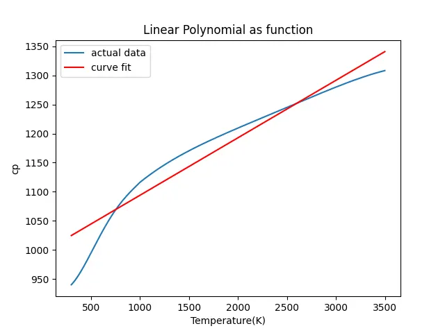
1.Graph for Linear Polynomial as function

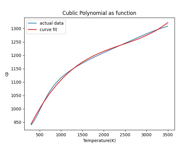
2.Graph for Cubic Polynomial as function

CONCLUSION

From the results we understands that the curve fits better when the degree of polynomial increases. If we further change the polynomial from cubic to quartic, the curve fit becomes much better than this case. We can understand from these figures that, the devaition between the actual data plot and function data plot decreased in the second case. Because in the second case we use the cubic polynomial equation as the function.