Vehicle Dynamics-Bump oscillation profile optimization using MATLAB

To calculate the following parameters, using the same front and rear spring rates for all three load conditions(Curb,Design and Gross vehicle weight).Front sprung mass natural frequency at half load can be consodered as `1.15Hz`.

• Recommended rear sprung mass frequency based on speed and wheelbase at half load condition.
• Front spring rate.
• Rear spring rate.
• Front sprung mass natural frequencies at curb and GVW.
• Rear sprung mass natural frequencies at curb and GVW.
• Front unsprung mass natural frequency at all three load conditions.
• Rear unsprung mass natural frequency at all three load conditions.
• Rear/Front frequency ratio for all three load conditions.

Notations used:

• GVW-Gross Vehicle weight
• `f_f`- front sprung mass frequency at half load in Hz.
• `f_r`- rear sprung mass frequency at half load in Hz.
• `f_{s_{f}}`- front sprung mass front frequency.
• `f_{s_{r}}`- front sprung mass rear frequency.
• `f_u`- frequency of unsprung mass.
• `k_{s_{f}}`- front spring rate.
• `k_{s_{r}}`- rear spring rate.

Given data:

Calculations:

• Rear spring mass frequency `f_r`:

Time lag `t_{l}=frac{text { wheelbase }}{text { speed }}=frac{2700 * 10^{-3}}{60 cdot(0.447)}=0.101s`

`f_{r}=1/((1/f_f)-t_l)=1/((1/1.15)-0.101)=1.301Hz`

• Front sprung mass frequency`f_{s_{f}}`:

It can be evaluated using `f_{s_{f}}=1/(2pi)sqrt(k_{r_{f}}/m_{s_{f}}`

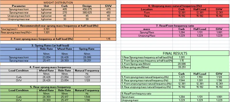
1. At curb natural frequency is 1.221 Hz

2. At GVW natural frequency is 1.128 Hz

• Rear sprung mass frequency `f_{r_{f}}`:

It can be evaluated using `f_{s_{r}}=1/(2pi)sqrt(k_{r_{r}}/m_{s_{r}}`

1. At curb natural frequency is 1.544 Hz

2. At GVW natural frequency is 1.196 Hz

Other calculations can be viewed in the below excel file:

(https://docs.google.com/spreadsheets/d/1-_9TX96mMyvk0drjtxUpS4zXUf3ri1k2/edit?usp=sharing&ouid=112677196525410410299&rtpof=true&sd=true)

Code:

% bump oscillation profile at half load

%weights in kg per corner
Ws_front = 456.875;
Ws_rear = 380.625;
Wu_front = 45;
Wu_rear = 30;

WB = 2700; %wheel base in mm
V = 60; %speed of vheicle in mph

%motion ratios
MR_f = 0.97;
MR_r = 0.85;

%time lag in sec
t1 = (WB*(10^(-3)))/(60*(0.447));

%recommended natural frequencies at half load
fs_front = 1.15;
fs_rear = 1/((1/fs_front)-t1);

%rates in N/mm
%tire rate (same for all)
kt = 245;

%ride rates
kr_front = (((fs_front*2*pi)^2)*(Ws_front))/1000;
kr_rear = (((fs_rear*2*pi)^2)*(Ws_rear))/1000;

%wheel rates
kw_front = (kt*kr_front)/(kt-kr_front);
kw_rear = (kt*kr_rear)/(kt-kr_rear);

%spring rates
ks_front = kw_front/(MR_f)^2;
ks_rear = kw_rear/(MR_r)^2;

%unsprung mass frequencies
fu_front = (1/(2*pi))*((kw_front+kt)*1000/Wu_front)^0.5;
fu_rear = (1/(2*pi))*((kw_rear+kt)*1000/Wu_rear)^0.5;

%plotting the graphs
%time range in sec
time = linspace(0,3.5,400);
i=1;
for t = linspace(0,3.5,400)
As_front(i) = exp(-t)*sin(2*pi*fs_front*t);
As_rear(i) = exp(-t)*sin(2*pi*fs_rear*(t-t1));
Au_front(i) = exp(-t)*sin(2*pi*fu_front*t);
Au_rear(i) = exp(-t)*sin(2*pi*fu_rear*(t-t1));
i=i+1;
end

figure(1)
subplot(2,1,1)
plot(time,As_front,'linewidth',2)
hold on
plot(time,As_rear,'linewidth',2)
title('Bump oscillation profile for Sprung mass at half load');
xlabel('Time (s)');
ylabel('amplitude (m)');
legend('Front','Rear');
grid on
subplot(2,1,2)
plot(time,Au_front,'linewidth',2);
hold on
plot(time,Au_rear,'linewidth',2);
title('Bump oscillation profile for Unsprung mass');
xlabel('Time (s)');
ylabel('amplitude (m)');
legend('Front','Rear');
grid on
saveas(1,'half _load', 'jpeg');

% bump oscillation profile at curb

%weights in kg per corner
Wsc_front = 405;
Wsc_rear = 270;
Wuc_front = 45;
Wuc_rear = 30;

%motion ratios
MR_f= 0.97;
MR_r = 0.85;

%spring rates
ksc_front = ks_front;
ksc_rear = ks_rear;

%wheel rates
kwc_front = ksc_front*(MR_f)^2;
kwc_rear = ksc_rear*(MR_r)^2;

%ride rates 
krc_front = (kt*kwc_front)/(kt+kwc_front); 
krc_rear = (kt*kwc_rear)/(kt+kwc_rear); 

%sprung mass frequencies
fsc_front = (1/(2*pi))*((krc_front*1000)/Wsc_front)^0.5; 
fsc_rear = (1/(2*pi))*((krc_rear*1000)/Wsc_rear)^0.5; 

%unsprung mass frequencies 
fuc_front = (1/(2*pi))*((kwc_front+kt)*1000/Wuc_front)^0.5; 
fuc_rear = (1/(2*pi))*((kwc_rear+kt)*1000/Wuc_rear)^0.5; 

%plotting the graphs 
%time range in sec 
time = linspace(0,3.5,400); 
j = 1; 

for tc = linspace(0,3.5,400) 
Asc_front(j) = exp(-tc)*sin(2*pi*fsc_front*tc); 
Asc_rear(j) = exp(-tc)*sin(2*pi*fsc_rear*(tc-t1)); 
Auc_front(j) = exp(-tc)*sin(2*pi*fuc_front*tc); 
Auc_rear(j) = exp(-tc)*sin(2*pi*fuc_rear*(tc-t1)); 
j=j+1; 
end 

figure(2) 
subplot(2,1,1)
plot(time,Asc_front,'linewidth',2,'color','red') 
hold on
plot(time,Asc_rear,'linewidth',2,'color','yellow')
title('Bump oscillation profile for Sprung mass at curb')
xlabel('Time (s)')
ylabel('Amplitude (m)') 
legend('Front','Rear') 
grid on 
subplot(2,1,2) 
plot(time,Auc_front,'linewidth',2,'color','red')
hold on 
plot(time,Auc_rear,'linewidth',2,'color','yellow')
title('Bump oscillation profile for Unsprung mass') 
xlabel('Time (s)') 
ylabel('Amplitude (m)') 
legend('Front','Rear') 
grid on 
saveas(2,'curb','jpeg') 

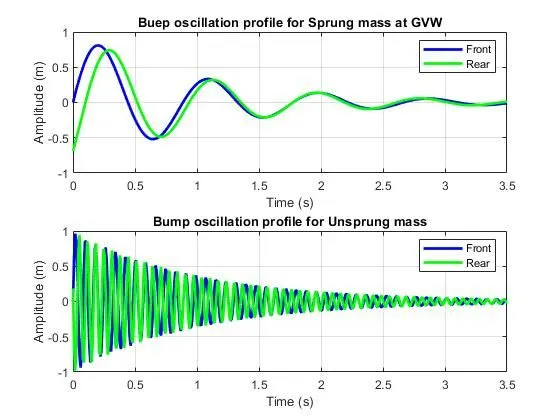
% bump oscillation profile at GVW 
%Weights in kg per corner 
Wsg_front = 475; 
Wsg_rear = 450; 
Wug_front = 45; 
Wug_rear = 30; 

%motion ratios 
MR_f= 0.97; 
MR_r=0.85;

%spring rates 
ksg_front = ks_front; 
ksg_rear = ks_rear; 

%Wheel rates 
kwg_front = ksg_front*(MR_f)^2;
kwg_rear = ksg_rear*(MR_r)^2; 

%ride rates
krg_front = (kt*kwg_front)/(kt+kwg_front); 
krg_rear = (kt*kwg_rear)/(kt+kwg_rear); 

%sprung mass frequencies
fsg_front = (1/(2*pi))*((krg_front*1000)/Wsg_front)^0.5; 
fsg_rear = (1/(2*pi))*((krg_rear*1000)/Wsg_rear)^0.5; 

%unsprung mass frequencies 
fug_front = (1/(2*pi))*((kwg_front+kt)*1000/Wug_front)^0.5;
fug_rear = (1/(2*pi))*((kwg_rear+kt)*1000/Wug_rear)^0.5; 

%plotting the graphs 
%time range in sec
time = linspace(0,3.5,400); 
k = 1; 
for tg = linspace(0,3.5,400)
    Asg_front(k)= exp(-tg)*sin(2*pi*fsg_front*tg); 
    Asg_rear(k) = exp(-tg)*sin(2*pi*fsg_rear*(tg-t1));
    Aug_front(k) = exp(-tg)*sin(2*pi*fug_front*tg);
    Aug_rear(k) = exp(-tg)*sin(2*pi*fug_rear*(tg-t1)); 
    k=k+1; 
end 

figure(3) 
subplot(2,1,1) 
plot(time,Asg_front,'linewidth',2,'color', 'blue');
hold on
plot(time,Asg_rear,'linewidth',2,'color','green');
title('Buep oscillation profile for Sprung mass at GVW'); 
xlabel('Time (s)') ;
ylabel('Amplitude (m)') 
legend('Front','Rear') 
grid on 
subplot(2,1,2) 
plot(time,Aug_front,'linewidth',2,'color','blue')
hold on 
plot(time,Aug_rear,'linewidth',2, 'color', 'green' )
title('Bump oscillation profile for Unsprung mass') 
xlabel('Time (s)')
ylabel('Amplitude (m)') 
legend('Front','Rear') 
grid on 

Conclusions:

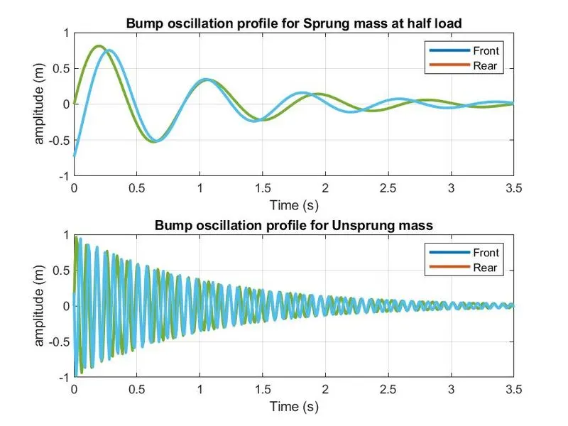
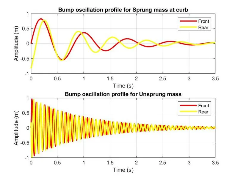
Bump oscillation profiles have been plotted for all three conditions. We can see from the graphs that the front and rear frequencies are almost in phase with each other at half load and GVW conditions, which means they are optimized.

1.Half load condition:

2.Curb condition:

3.GVW condition: